Wave equation modeling can be regarded as a linear operator, the domain of the operator is a the scattering field, and the range is a seismic dataset. When the scattering field and seismic data are discretized they can be represented as finite dimensional vectors. The modeling operator, A, maps from a scatterer vector, s to a data vector d.
As = d
When imaging we wish to obtain an estimate of s from the measured data d. One possible operation is to apply the adjoint operator,![]()
![]()
If a conjugate gradient algorithm is used the application of the adjoint can be regarded as the first iteration of that algorithm.
Another method for obtaining an estimate is to note that the solution of the least squares problem is given by
![]()
| |
(8) |
This procedure can also be interpreted as the first step of an iterative algorithm. In this case the problem being solved is a preconditioned version of the original problem. M = ( Diag(A'A) )-1/2 is a diagonal preconditioner that equalizes the norm of the columns of the operator A. The preconditioned least squares problem is,
 |
(9) | |
| (10) |
In many applications it is relatively simple to calculate ( Diag(A'A) ). For the modeling algorithm used here it is,
![]()
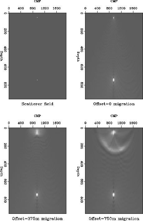
If the modeling is not limited in spatial aperture, the weight is just a function of depth and offset panel. It is a depth and offset dependent scale applied after adjoint modeling rather than the time dependent scale usually applied before migration in seismic processing.
Figure ![[*]](http://sepwww.stanford.edu/latex2html/cross_ref_motif.gif) shows the constant offset migrations
calculated using this weight function. The amplitudes of the two
scatterers have been correctly recovered. The diagonal weight only
corrects the relative amplitudes of the result, it does not correct the
spectrum of the result, the full inverse operator (A'A)-1A' would
correct the spectrum as well.
shows the constant offset migrations
calculated using this weight function. The amplitudes of the two
scatterers have been correctly recovered. The diagonal weight only
corrects the relative amplitudes of the result, it does not correct the
spectrum of the result, the full inverse operator (A'A)-1A' would
correct the spectrum as well.
 |