


P- and SV-wave
synthetic traveltimes were generated using the anisotropic ray tracing
algorithm described in Michelena (1992b).
Figure ![[*]](http://sepwww.stanford.edu/latex2html/cross_ref_motif.gif) shows
the heterogeneous TI model where the rays were traced.
This model shows the variation in depth of
shows
the heterogeneous TI model where the rays were traced.
This model shows the variation in depth of ![]() ,the elastic
constants transformed to velocity assuming unit density.
The cross-well geometry used to compute the traveltimes
consists of 92 sources and 92 receivers
at each well. The distance between wells is 390 feet, and the
separations between consecutive sources or receivers is 23 feet.
,the elastic
constants transformed to velocity assuming unit density.
The cross-well geometry used to compute the traveltimes
consists of 92 sources and 92 receivers
at each well. The distance between wells is 390 feet, and the
separations between consecutive sources or receivers is 23 feet.
|
elastic-exacto
Figure 1 Layered TI synthetic model. From left to right the four curves represent the elastic constants in units of velocity V44, V13, V33, and V11, respectively. The density is assumed to be unity. | 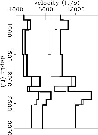 |

Since the elastic constants of the medium are known, the corresponding
elliptical velocities (VP,x, ![]() , VSV,x, and
, VSV,x, and
![]() ) can be calculated easily by using the equations derived in
Michelena (1992c).
Figure shows the result.
These velocities can be used to check
how the algorithm performs in the first step toward the estimation
of the elastic constants, that is, the tomographic
estimation of the elliptical
velocities.
) can be calculated easily by using the equations derived in
Michelena (1992c).
Figure shows the result.
These velocities can be used to check
how the algorithm performs in the first step toward the estimation
of the elastic constants, that is, the tomographic
estimation of the elliptical
velocities.
The paraxial elliptical approximation around the
horizontal axis (assuming vertical axis of symmetry)
is accurate for angles of less than 30 degrees (Michelena, 1992c). For this
reason, the inversion only uses rays whose angle measured
from the horizontal satisfies this condition.
However, no approximation
is
made in the computation of the synthetic traveltimes
through the model of Figure .
The paraxial approximation is made only
during the inversion procedure in which the rays
are traced in elliptically anisotropic instead of transversely
isotropic models.
The fact that the straight line that connects a source-receiver pair forms a small angle with respect to the horizontal doesn't necessarily mean that the angle of the corresponding ray path is also small. The angle of the ray path increases in low-velocity layers and
|
syn-ellip
Figure 2 Theoretical elliptical velocities around the horizontal axis calculated from the elastic constants shown in Figure 1. From left to right the four curves represent VSV,x, | 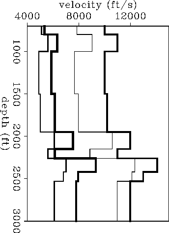 |
decreases in high-velocity layers. However, if the velocity contrasts are not too strong, it should be enough to look at the straight line that connects source and receiver to select the rays that satisfy the proper constraints.
Figure
shows the result of inverting the P-wave traveltimes.
This figure also shows
the theoretical elliptical velocities calculated from the elastic constants.
The estimation of the horizontal P-wave velocity
is, as expected, almost perfect, whereas the vertical NMO velocity is
slightly overestimated (![]() ) in all layers.
As Figure shows,
the estimation
of the vertical NMO velocity is more accurate
when inverting
SV-wave traveltimes
than when
inverting P-wave traveltimes,
which means that, for the range
of ray angles used, the elliptical approximation works better
for SV-waves than
for P-waves. The error in
) in all layers.
As Figure shows,
the estimation
of the vertical NMO velocity is more accurate
when inverting
SV-wave traveltimes
than when
inverting P-wave traveltimes,
which means that, for the range
of ray angles used, the elliptical approximation works better
for SV-waves than
for P-waves. The error in ![]() is less
than one percent.
is less
than one percent.
The errors in the NMO velocities ![]() and
and ![]() come from
using an elliptical approximation for ray angles that are not sufficiently
small. When the model is truly elliptical, the estimation
of the NMO velocities is accurate.
come from
using an elliptical approximation for ray angles that are not sufficiently
small. When the model is truly elliptical, the estimation
of the NMO velocities is accurate.
|
syn-ellip-p
Figure 3 P-wave elliptical velocities. Dashed lines: result of the inversion of P-wave traveltimes with a ray angle of less than 30 degrees. Continuous lines: theoretical values. The curves with lower velocity correspond to | 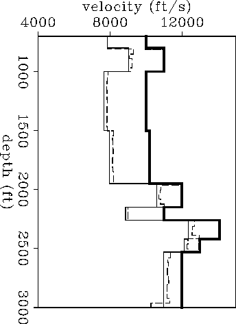 |
|
syn-ellip-s
Figure 4 SV-wave elliptical velocities. Dashed lines: result of the inversion of SV-wave traveltimes with a ray angle of less than 30 degrees. Continuous lines: theoretical values. The curves with lower velocity correspond to VSV,x, and the ones with higher velocity correspond to |  |
The variation
with depth in the
theoretical P- and SV-wave elliptical velocities
has
been estimated accurately. Therefore, by using these two
models of elliptical velocities,
we can also expect an accurate estimation of the elastic constants,
as Figure shows.
Since P- and SV-wave traveltimes are inverted separately and the
interfaces are not constrained to move consistently with both data sets,
the models obtained for P- and SV-wave
elliptical velocities may not
have all the interfaces at exactly the same depths.
As a consequence, artificial thin layers (spikes) may
appear when we estimate the elastic constants because there may be slight
relative mispositions of the same boundaries in the two models.
In Figure
these spikes are removed by applying a median filter to the
elastic constants after the mapping from elliptical velocities.
Another way to solve this problem is by
describing the interfaces with the same parameters for both
P- and SV-wave velocity models and inverting the two sets of traveltimes
simultaneously.
Depending on the radiation pattern of the source, traveltimes
that correspond to nearly horizontal rays may not always be
available for either P- or SV-waves. When this happens,
it may be necessary to use
ray angles that are far from the horizontal because nothing
else is available.
Figure shows an example
where SV-wave elliptical velocities
have been
estimated by using ray angles between 28 and 36
degrees. The estimated horizontal component of the velocity
is as accurate as in Figure even though this
component is not
well sampled by the ray paths used. The
error in ![]() increases when using larger ray angles.
However, as Figure indicates,
the error in the estimation of the elastic
constants is still
small because the P-wave elliptical velocities
were estimated using small ray angles.
increases when using larger ray angles.
However, as Figure indicates,
the error in the estimation of the elastic
constants is still
small because the P-wave elliptical velocities
were estimated using small ray angles.
|
exact-vs-approx-median
Figure 5 Elastic constants that control P- and SV-wave propagation. Dashed lines: estimated. Continuous lines: given. From left to right the four pairs of curves represent V44, V13, V33, and V11, respectively. | 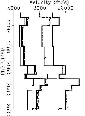 |
|
syn-ellip-s-28to36
Figure 6 SV-wave elliptical velocities. Dashed lines: result of the inversion of SV-wave traveltimes with ray angles between 28 and 36 degrees. Continuous lines: theoretical SV-wave elliptical velocities. The curves with lower velocity correspond to VSV,x and the ones with higher velocity correspond to | 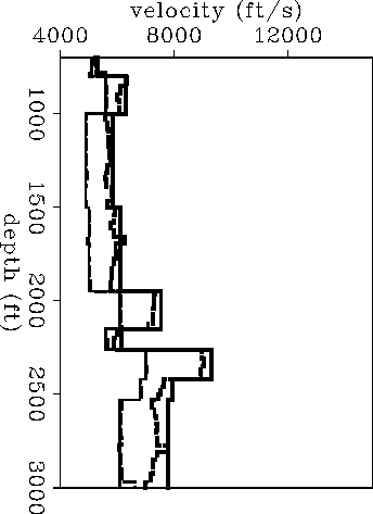 |
|
exact-vs-approx-28to36
Figure 7 Elastic constants that control P- and SV-wave propagation. Dashed lines: elastic constants estimated when the ray angles used in the tomographic inversion of SV-wave traveltimes are between 28 and 36 degrees. The ray angles used to obtain the P-wave elliptical velocities are between 0 and 30 degrees, as in Figure 5. Continuous lines: original elastic constants. From left to right the four pairs of curves represent V44, V13, V33, and V11, respectively. |  |
In the field data example that follows, SV-wave traveltimes are not available for small vertical offsets.