The equivalence of the constrained two-D filter and FX-decon

The similarity in the results of applying Filter (2) and applying FX-decon may be explained by the Fourier transform of the FX-decon operators. FX-decon calculates a separate filter within each frequency of the form  

$$\begin{array} {ccccc} 1 & a_{2} & a_{3} & a_{4} & a_{5} \end{array}.$$ (3)

If these filters were transformed from the frequency-space domain into the time-space domain, they would appear as a single two-dimensional filter. The collection of these filters in the frequency-space domain $\begin{array} {ccccc} 1 & a & a & a & a \\ 1 & a & a & a & a \\ 1 & a & a ... ...a \\ 1 & a & a & a & a \\ 1 & a & a & a & a \\ 1 & a & a & a & a \end{array}$transforms to $\begin{array} {ccccc} \cdot & a & a & a & a \\ \cdot & a & a & a & a \\ \cd... ...& a & a & a & a \\ \cdot & a & a & a & a \\ \cdot & a & a & a & a \end{array}$in the time-space domain, where the number of rows is the number of time samples in the window being considered. (The subscripts are omitted for simplicity.) The previous time-space filter is the same as Filter (2) except for the number of rows. It might be expected that the prediction would be limited to elements close to the center of the filter, since events far from the output point are unlikely to affect data at the output position, but correlations for events widely separated in time will create problems with incorrect lineups in the output of FX-decon.

To keep the calculation and application of the filters symmetrical, the two-dimensional deconvolution examples shown in this paper have two filters calculated and applied within each window: one forward in space and one reversed. The filters are not extended beyond times where a full filter response is available, so the two-dimensional deconvolution results shown here have the original data at the top and bottom of the section.

For the type operator shown in Filter (1), the filter calculated for the forward prediction was  

$$\begin{array} {ccccc} 0.4564 & -0.2629 & -0.01173 & 0.1009 ... ....04788 \\ 0 & 0.1422 & 0.06668 & 0.06372 & 0.04849 \end{array}$$ (4)

and for the reverse prediction, the filter calculated was  

$$\begin{array} {ccccc} 0.4958 & 0.004744 & 0.03781 & 0.07075... ...5511 \\ 0 & -0.2811 & -0.1534 & 0.02327 & 0.05016 \end{array}.$$ (5)

For simplicity, I will refer to this type of filter, with free coefficients in the output column, as the a₁₁-free filter.

For a filter of the type shown in Filter (2), the filter calculated appears as  

$$\begin{array} {ccccc} 0 & -0.2853 & -0.1097 & 0.05663 & 0.0... ...0.02693 \\ 0 & 0.1136 & 0.02811 & 0.0521 & 0.03426 \end{array}$$ (6)

for the forward prediction, and  

$$\begin{array} {ccccc} 0 & 0.1136 & 0.02811 & 0.0521 & 0.034... ...02693 \\ 0 & -0.2853 & -0.1097 & 0.05663 & 0.02574 \end{array}$$ (7)

for the reverse prediction. I will refer to this filter as the a₁₁-constrained filter.

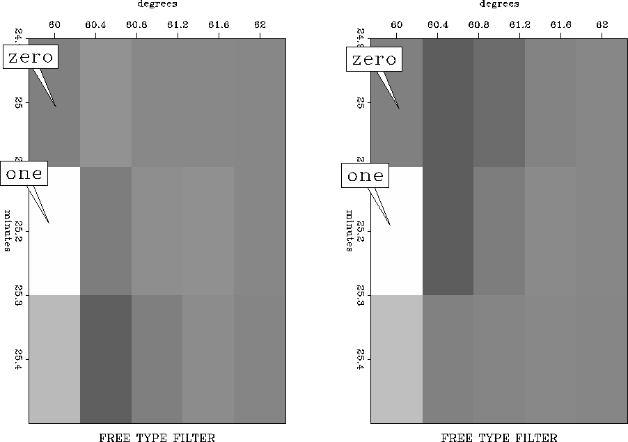
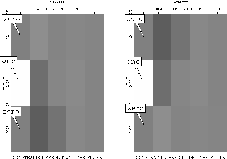
Notice that the forward and reverse predictions are symmetric in the case of the a₁₁-constrained type filter but not for the a₁₁-free filter. Plots of the filters are shown in Figures 1 and  2.

 

lomofilt
Figure 1 A calculated a₁₁-free filter. The left side is the forward filter, and the right side is the reverse filter. Push the button for a movie of the filters for each iteration of the filter design process.

 

latrfilt
Figure 2 A calculated a₁₁-constrained filter. The left side is the forward filter, and the right side is the reverse filter. Push the button for a movie of the filters for each iteration of the filter design process.

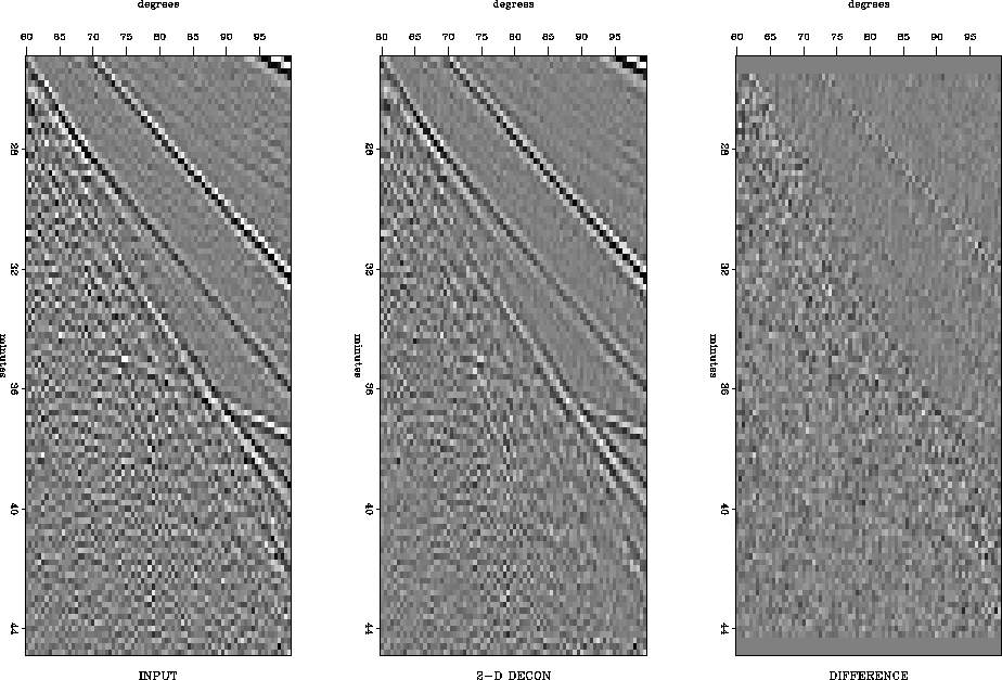
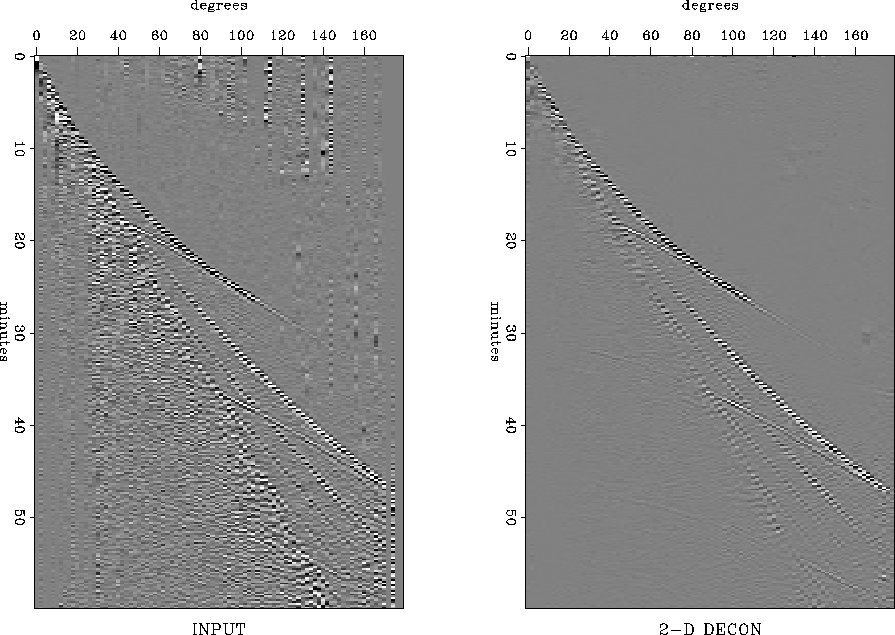
Now compare the results of the previous two filter shapes on the data that show the greatest difference when used with the a₁₁-free filter and the a₁₁-constrained filter. The result using the a₁₁-constrained filter is shown in Figure 3. The a₁₁-free filter result is shown in Figure 4. Figure 4 shows that the a₁₁-free filter has passed much more noise than the a₁₁-constrained filter. Finally, we show Shearer's full dataset in Figure 5. The two-dimensional deconvolution filter using the a₁₁-constrained filter has eliminated most of the random noise in the input section. Examples of comparisons between FX-decon and lateral prediction with two-dimensional deconvolution are shown in another paper in this volume Abma (1993).

 

trans
Figure 3 Two-D deconvolution filtering of the horizontal component of Shearer's global image dataset with the a₁₁-constrained filter.

 

transy
Figure 4 Two-D deconvolution filtering of the horizontal component of Shearer's global image dataset using the a₁₁-free filter.

 

s2D
Figure 5 Two-dimensional deconvolution filtering of the horizontal component of the full global image dataset using the a₁₁-constrained filter. Push the button to change the processing parameters and plot a new version of the output.