Next: CONCLUSIONS
Up: Abma: Lateral prediction
Previous: TWO-D DECONVOLUTION FILTERING
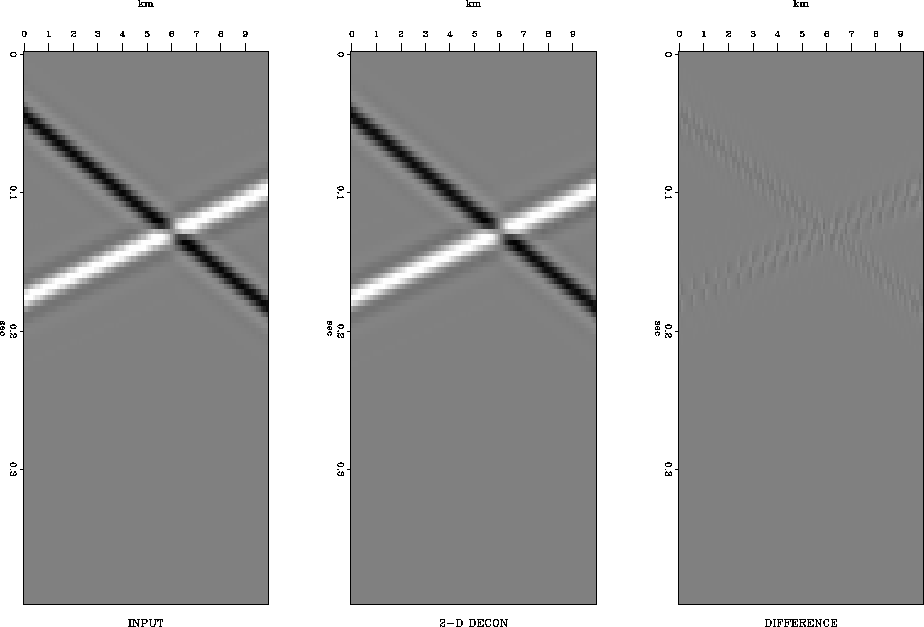
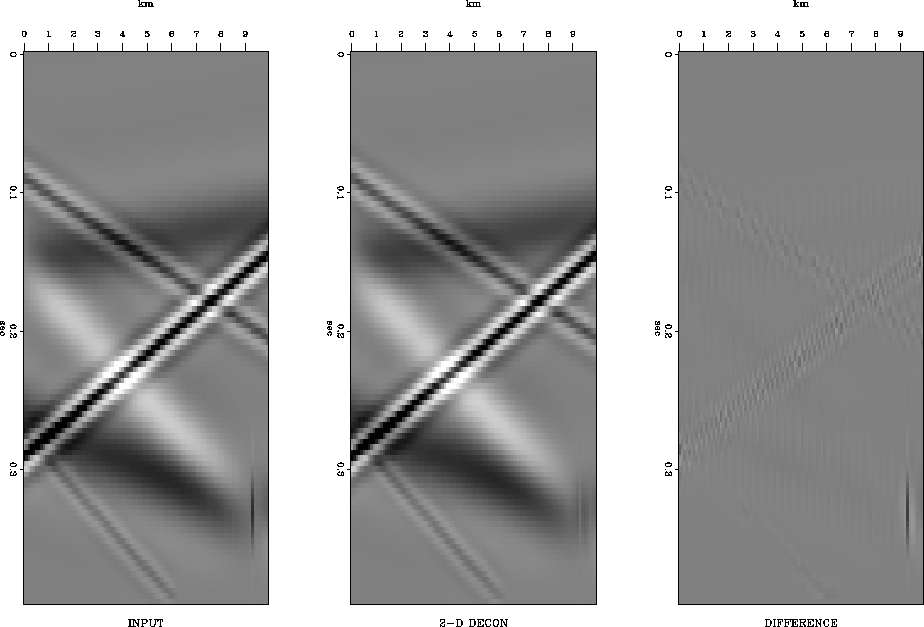
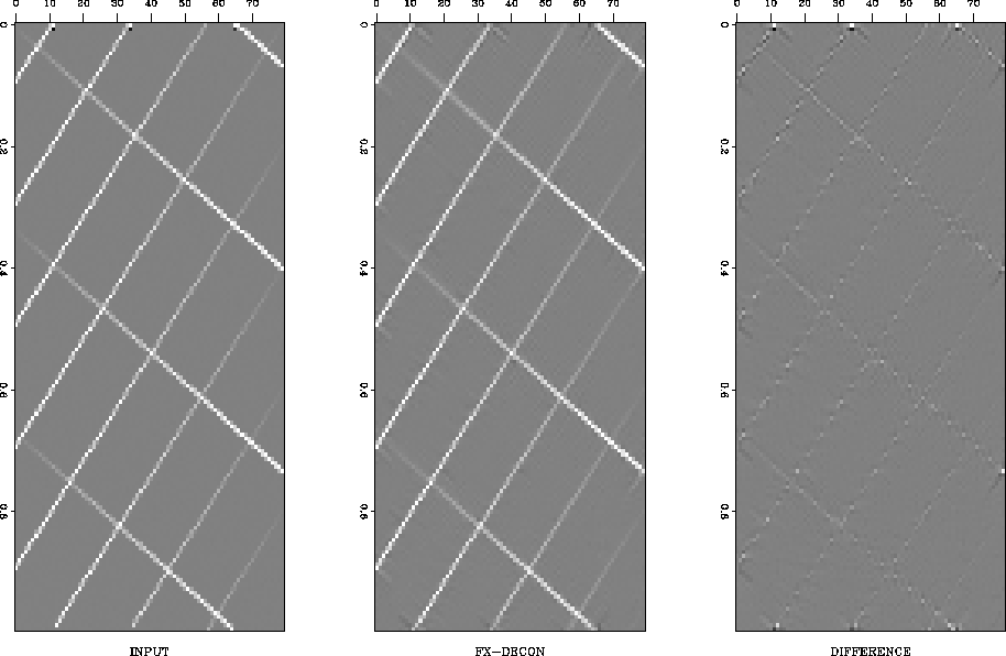
A simple two-dip example shows that both
FX-decon and two-dimensional deconvolution retain the original signal.
Figure 2 and Figure 3 compare the results of
two-dimensional deconvolution and FX-decon
in the noiseless case. The
weak events seen in the
difference sections are the result of
the sampling used in creating the dipping events. Flat events may be
completely removed using either of these techniques.
dips
Figure 2
Two-D prediction-error filtering


 dipsfx
Figure 3
FX-decon filtering
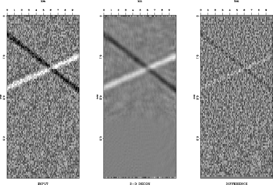
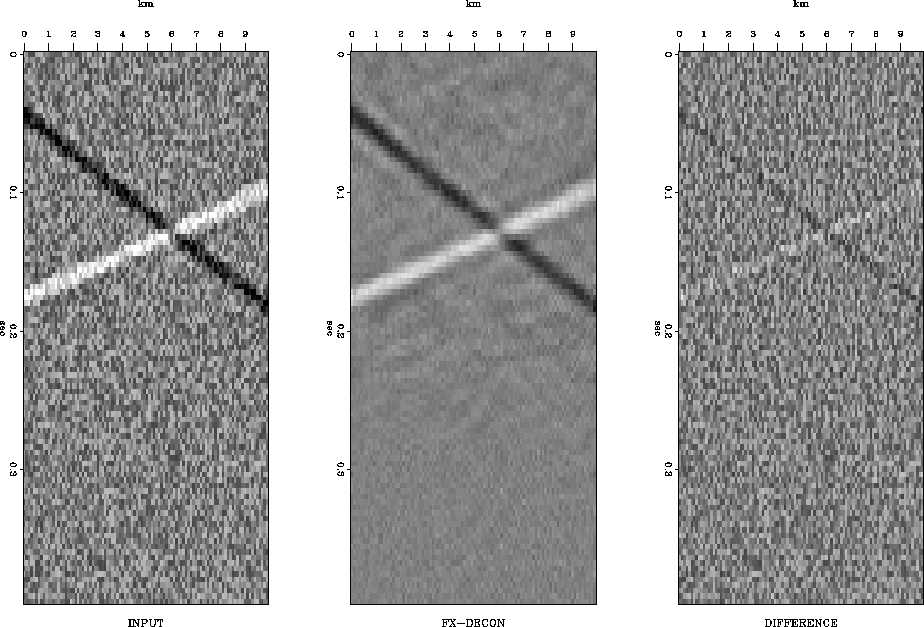
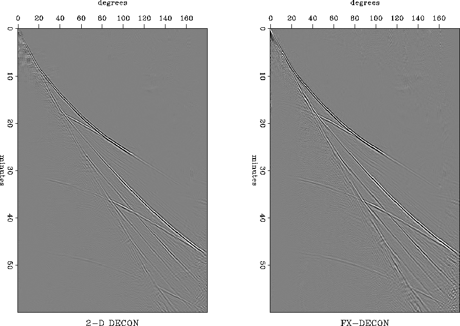
When noise is added, FX-decon and two-dimensional deconvolution
show similar results, as seen in Figures 4 and 5.
The noise is significantly attenuated, and the
linear events are retained. Notice that the two-dimensional deconvolution
removes more noise than FX-decon
in the lowest window where no signal is present.
Three windows in time and four windows in x with fifty percent overlap
are used in Figures 4 and 5.
The noise remaining at the top and bottom of the prediction section of
Figure 4
is the original data, since the output is not predicted unless the filter
covers a full set of data. This may be remedied by saving the
filter after it is calculated and then applying it to a wider range of data.
In this version of the two-dimensional deconvolution program,
the calculation of the filter and the filtering is performed
simultaneously.
noise
Figure 4
Two-D prediction-error filtering. Notice how weak the noise is on the
lower part of the output compared to Figure 5. The original data are
output at the top and bottom because
the filters have not been applied past the edges there.
noisefx
Figure 5
FX-decon filtering. Notice how strong the noise is on the
lower part of the output compared to Figure 4.
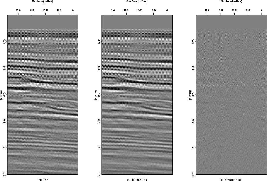
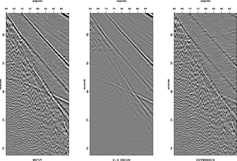
Both processes applied to real data again show that the results
are similar, as seen in Figures 6 and 7.
In the shallow section, both filters have predicted the
even-odd effect, where alternate traces have different amplitudes, since
both filters can predict it.
There were 16 overlapping windows in time and three windows in x
in these examples.
WGstack
Figure 6
Two-D prediction-error filtering applied to a Gulf of Mexico line.
WGstackfx
Figure 7
FX-decon filtering applied to a Gulf of Mexico line.
The previous similarities between the processes are seen in the global image
of
a portion of a dataset created by Shearer1991
seen in Figures 8 and 9.
Notice that there is some lineup of the noise with strong events
in Figure 9.
Otherwise, the FX-decon appears to do as well as
two-dimensional deconvolution.
A comparison using the full dataset is shown in Figure 10.
transverse
Figure 8
Two-D deconvolution filtering of the horizontal component
of Shearer's global image dataset. There is less ringing here than
in Figure 9.
transversefx
Figure 9
FX-decon filtering of the horizontal component
of Shearer's global image dataset. There is more ringing here than
in Figure 8.
s2Dfx
Figure 10
Two-D deconvolution and FX-decon of the horizontal component
of Shearer's global image dataset. Two-D deconvolution has passed
less noise and produced fewer artificial lineups.
More significant differences are seen when 2-dimensional deconvolution
and FX-decon are applied to random noise. The predictions shown by
Figures 11 and 12
are seen to have lined up some of the random noise, but the
FX-decon has left more noise than the two-dimensional deconvolution. This may
be attributed to the greater degree of freedom FX-decon has in
making predictions and to the extended length of the filter in the time domain.
rnoise
Figure 11
Random noise with two-D prediction filtering. There is
less noise on output than seen in the comparable FX-decon output
seen in Figure 12.
rnoisefx
Figure 12
Random noise with FX-decon filtering. There is
more noise on output than seen in the comparable two-D prediction filter
output seen in Figure 11.
FX-decon applies a prediction process to each frequency separately,
while two-dimensional prediction-error filtering generates a single filter
for each window.
Figures 13 and 14
show the results of creating three dipping events with a high-cut frequency of
15 Hz. and another three dipping events
with a low-cut of 35 Hz. and a high-cut of 60 Hz.
While some differences may be expected when applied
to events with different frequency ranges, the differences between the
results are found to be small.
fdips
Figure 13
Dips of different frequency content with two-D prediction-error filtering
fdipsfx
Figure 14
Dips of different frequency content with FX-decon filtering
Events with amplitudes that vary spatially, even in what seems to
be a predictable manner, tend not to be predicted well by either
technique. Figures 15 and 16 show the comparisons.
The weak events seen following the events in Figure 15
are caused by the finite width of the filter and the zeroed background.
The main energy in Figure 15 is the same as Figure 16.
Here, FX-decon may be considered to have a slightly better prediction,
but no major differences are seen.
conflict
Figure 15
Two-D prediction-error filtering applied to
conflicting events with changing amplitudes.
conflictfx
Figure 16
FX-decon filtering applied to
conflicting events with changing amplitudes.
Next: CONCLUSIONS
Up: Abma: Lateral prediction
Previous: TWO-D DECONVOLUTION FILTERING
Stanford Exploration Project
11/17/1997