


FX-decon is a simple process that predicts linear events by making predictions in the frequency-space domain.
The FX-decon prediction process depends on the form of linear events
in frequency versus x, x being the space direction. Given a linear event,
![]() , the Fourier transform of this event is
, the Fourier transform of this event is
![]() or
or ![]() . In x, the function is clearly
periodic. To predict a linear event, a least squares prediction filter
is calculated, using
. In x, the function is clearly
periodic. To predict a linear event, a least squares prediction filter
is calculated, using ![]() where f is the
prediction filter, d is the desired output, and X is a matrix filled
with shifted versions of the input series in x.
where f is the
prediction filter, d is the desired output, and X is a matrix filled
with shifted versions of the input series in x. ![]() indicates the
transpose conjugate.
indicates the
transpose conjugate.
Following the nomenclature of
Gulunay1986,
d is the data shifted by one sample, or
![]() .The input data,
.The input data,
![]() ,forms the matrix X below:
,forms the matrix X below:
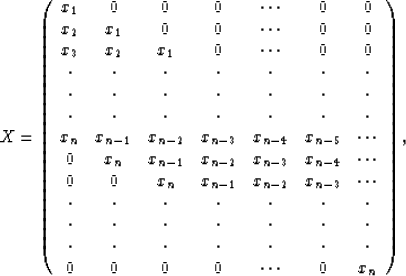 |
(1) |
The process of applying FX-decon starts by partitioning the data into windows small enough so events of interest appear linear. The data within each window are then Fourier transformed. For each frequency, a prediction filter is calculated and applied twice; once forward in space and once backwards. The two predictions are summed, the inverse Fourier transform applied, and the windows merged back into the output. Note that the operations within each frequency are independent of other frequencies. This allows a large degree of freedom in the prediction of the output.
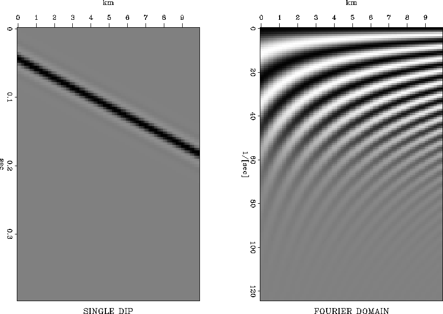
Another interesting feature of the FX-decon process pointed out by Spitz 1991 involves the relationships of the response of a dip at one frequency to that at another frequency. In Figure 1, a single dipping event is shown in time and after Fourier transformation of the time axis. It can be seen that the events are periodic both in frequency and in space. The periodicity at low frequency may be used to predict the shape of the higher frequency components and may be used to guide interpolation of events that are aliased in the high frequency components, but not aliased at low frequencies.
 |


