The qdome synthetic

Earlier 2-D migration and LOMOPLAN studies such as 1992b used a model called ``Sigmoid''. I used the sigmoid model for several applications and others also found it useful Zhang and Claerbout (1992). Using the same modeling concepts, I set out to make a three-dimensional model. The model has horizontal layers near the top, a Gaussian appearance in the middle, and dipping layers on the bottom with horizontal unconformities between the three regions. 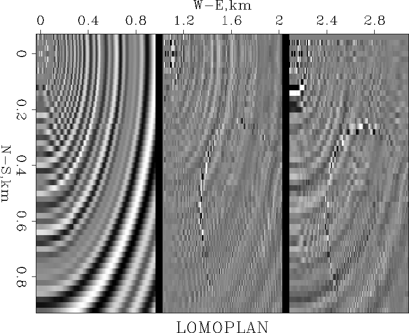Figure 1 shows a vertical slice through the 3-D ``qdome'' model and components of its LOMOPLAN. There is also a fault that will be described later.

 

qdomesico
Figure 1 Left is a vertical slice through the 3-D ``qdome'' model. Center is the in-line component of the LOMOPLAN. Right is the cross-line component of the LOMOPLAN.

The most interesting part of the qdome model is the Gaussian center. I started from the equation of a Gaussian

$$z(x,y,t) \quad = \quad e^{-(x^2+y^2)/ t^2}$$ (2)

and backsolved for t

$$t(x,y,z) \quad = \quad \sqrt{x^2+y^2 \over -\ln z}$$ (3)

Then I used a random number generator to make a blocky one-dimensional impedance function of t. At each (x,y,z) location in the model I used the impedance at time t(x,y,z), and finally defined reflectivity as the logarithmic derivative of the impedance. Without careful interpolation (particularly where the beds pinch out) a variety of curious artifacts appear. I hope to find time to make a tutorial lesson on interpolation from the experience of making the qdome model. As a refinement to the model, within a certain subvolume the time t(x,y,z) is given a small additive constant. This gives a fault along the edge of the subvolume. Ray Abma defined the subvolume for me in the qdome model. The fault looks quite realistic, and it is easy to make faults of any shape, though I wonder how they would relate to realistic fault dynamics. Figure 2 shows a top view of the 3-D qdome model and components of its LOMOPLAN.

Notice the cross-line spacing has been chosen to be double the in-line spacing. Evidently a consequence of this in both Figure 1 and Figure 2 is that the Gaussian dome is not so well suppressed on the crossline cut as on the in-line cut. By comparison, notice that the horizontal bedding above the dome is perfectly suppressed, whereas the dipping bedding below the dome is imperfectly suppressed.

 

qdometoco
Figure 2 Left is a horizontal slice through the 3-D qdome model. Center is the in-line component of the LOMOPLAN. Right is the cross-line component of the LOMOPLAN. Press button for volume view.

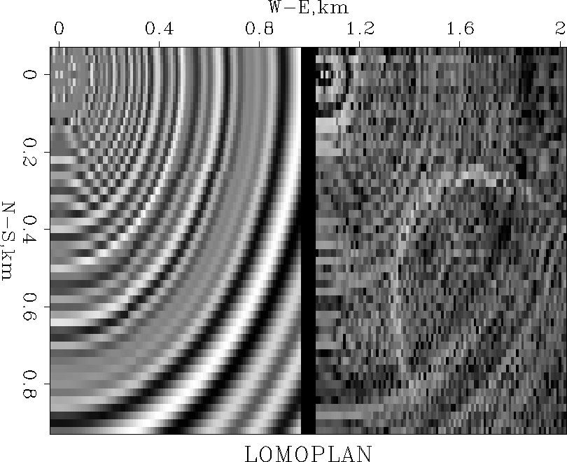
Finally, I became irritated at the need to look at two output volumes. Since I rarely if ever interpreted the polarity of the LOMOPLAN components, I formed their sum of squares and show the square root in Figure 3.

 

qdometora
Figure 3 Left is the model. Right is the magnitude of the LOMOPLAN components in Figure 2. Press button for volume view.