previous up next print clean
Next: Further Study Up: Oh: Transmissivity In Fine Previous: Markov Chain

TRANSMISSIVITY SIMULATION

To model a one dimensional medium, additive quantities such as density and compliance are assigned to the random sequences made in the previous section. In this case, only two states are considered. The equations needed for simulation are taken from the paper by Muir in this report. The equations for crossing the boundary of the two different states are,
\begin{displaymath}
\pmatrix{
 v \cr
 \sigma}
 = \pmatrix{
 1 & 1 \cr
 \sqrt{\rho/s} & - \sqrt{\rho/s}}
 \pmatrix{
 v^{+} \cr
 v^{-}}\end{displaymath} (3)
\begin{displaymath}
\pmatrix{
 v^{+} \cr
 v^{-}}
 =
 \frac{1}{2}
 \pmatrix{
 1 & \sqrt{s/\rho} \cr
 1 & -\sqrt{s/\rho}}
 \pmatrix{
 v \cr
 \sigma}\end{displaymath} (4)
and the translation equation within a layer of thickness z, density $\rho$ and compliance s is,
\begin{displaymath}
\pmatrix{
 v^{+}(z) \cr
 v^{-}(z) }
 =
 \pmatrix{
 e^{-i \om...
 ...+i \omega z \sqrt{\rho s}}}
 \pmatrix{
 v^{+}(0) \cr
 v^{-}(0)}\end{displaymath} (5)
These three equations can be combined to form a basic building block  
 \begin{displaymath}
\pmatrix{
 v(z) \cr
 \sigma(z) }
 =
 \pmatrix{
 \cos(\omega ...
 ... \cos(\omega z \sqrt{\rho s})}
 \pmatrix{
 v(0) \cr
 \sigma(0)}\end{displaymath} (6)

where

v : velocity field

$\sigma$ : traction field

v+ : upgoing wave amplitude

v- : downgoing wave amplitude

z : layer thickness

$\rho$ : density of each layer

s : compliance of the layer

Let ${\bf A}_{i}$ a building block matrix in i-th layer. Then,  
 \begin{displaymath}
{\bf A}_{i}=
 \pmatrix{ 
 \cos(\omega z_{i} \sqrt{\rho_{i} s...
 ...t{\rho_{i} s_{i}}) &
 \cos(\omega z_{i} \sqrt{\rho_{i} s_{i}})}\end{displaymath} (7)
By multiplying the matrices ${\bf A}_{i}$ for all layers, we get the following solution of the transmissivity T in the frequency domain.
\begin{displaymath}
\pmatrix{
 T \cr
 0 }
 =
 \frac{1}{2}
 \pmatrix{
 1 & \sqrt{...
 ... 1 \cr
 \sqrt{\rho/s} & - \sqrt{\rho/s}}
 \pmatrix{
 I \cr
 R }\end{displaymath} (8)

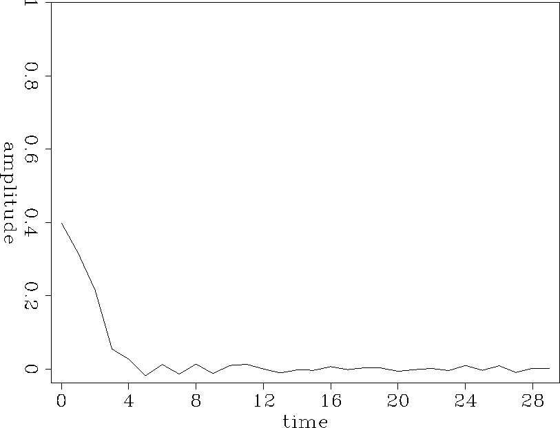
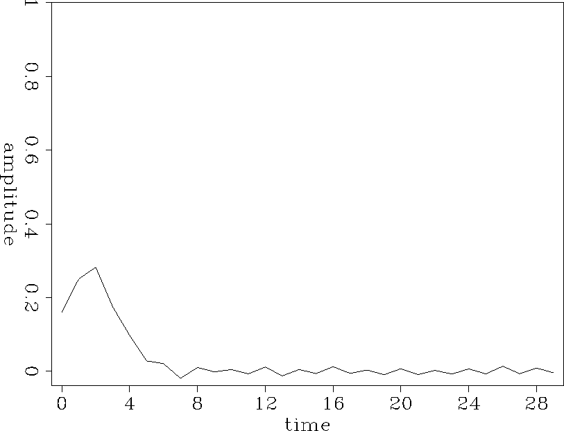
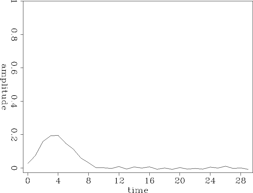
An impulse of amplitude 1 is used as an input. The output is averaged over 32 different random sequences with the same statistical properties. The experiment is done for various numbers of layers to see how the number of layers affects the output. The numbers used here are powers of 2, say 32,64,128. To make problem simpler, the velocities of the two states are chosen to be the same. The time sampling interval is equal to the difference between the arrival time of the primary and that of the shortest path multiple. The frame is retarded by the amount of the first arrival time. Figure 1-4 show the impulse responses for the different four numbers of layers.

 
avrg16
avrg16
Figure 1
Impulse response for 16 layers
view

 
avrg32
avrg32
Figure 2
Impulse response for 32 layers
view

 
avrg64
avrg64
Figure 3
Impulse response for 64 layers
view

 
avrg128
avrg128
Figure 4
Impulse response for 128 layers
view

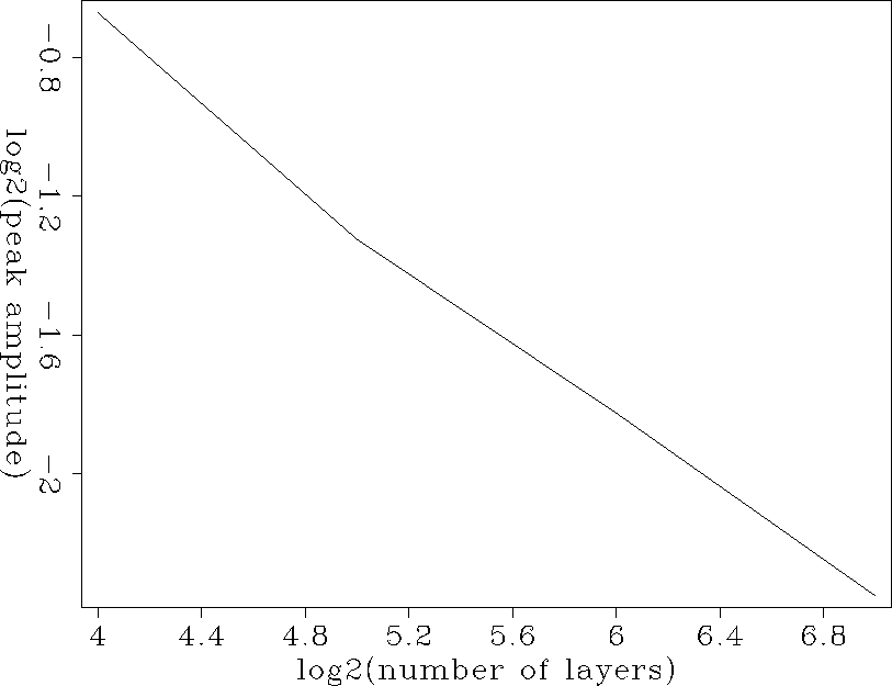
As expected, the impulse broadens as the number of layers increases. The peak arrival time is retarded accordingly. The peak amplitude decays approximately in proportion to the square root of the number of layers. Figure 5 shows this relationship. The retarded time of the peak amplitude from the primary is proportional to the number of the layers.
 
amp-num
amp-num
Figure 5
The peak amplitude decays in proportion to approximately square root of number of layers.
view


previous up next print clean
Next: Further Study Up: Oh: Transmissivity In Fine Previous: Markov Chain
Stanford Exploration Project
11/17/1997