A MODEL PROBLEM

To illustrate the various interpolation techniques I will use a 2-D surface that is a plane wave of frequency, $\omega$, and slowness, p,

$$f(x,t) = sin( \omega ( t - p x ) ).$$

This function is shown in Figure  for a frequency of 20Hz and a slowness of 1/2000 $\rm ms^{-1}$.

 

raw-func
Figure 1 Example continuous data, a mono-frequency plane wave with frequency 20Hz and slowness 1/2000 $\rm ms^{-1}$.

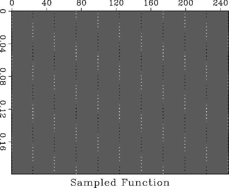
If this data is sampled using typical seismic data sampling rates, 4ms in time and 25m in space, the data shown in figure  is obtained. This is the input data to the various interpolation schemes,

$$\tilde{f}(ix,it) = f(x_{ix},t_{it})\,;\ ix \in \{1,\ldots,nx \}, it \in \{1,\ldots,nt\}$$

The data is sampled at coordinates given by x_ix and t_it.

 

sampled-func
Figure 2 Input data sampled every 4ms in time and 25m in space.

In the following examples I consider the case of an integral path on a 2-D surface that is defined by time as a function of space, t(x). The aim of this paper is to obtain the integral along a particular path as the sum over all the traces of the trace scaled by a weighting function which is localized around the intersection of the integration trajectory and each trace, t(x_ix), with nearest sample point it(ix). The curve integral can then be expressed as a sum over the sampled data points.

$$\int_{xmin}^{xmax} f( x, t(x) ) \, dx = \sum_{ix=1}^{nx} \, \sum_{j=-n}^{+m} w(ix,it,j) \tilde{f}(ix,it(ix) + j)$$