


The representation of a velocity field is crucial to the accuracy and efficiency of traveltime and amplitude calculations. Because the traveltime and amplitude calculations are more accurate in a continuous velocity model than in a discontinuous velocity model, I map a given velocity field onto a grid formed by regular triangular cells. Within each triangular cell, velocity varies linearly, as follows:
| v(x,z) = vo+vx(x-xo)+vz(z-zo), | (1) |
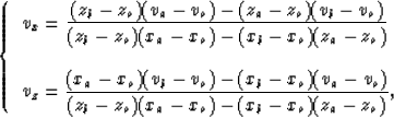 |
(2) |
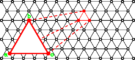
![[*]](http://sepwww.stanford.edu/latex2html/cross_ref_motif.gif) shows examples of a triangular grid and
a triangular cell. With this representation, velocity is continuous
everywhere, including
the boundaries of adjacent triangular cells.
Velocity contrasts at the interfaces
of the original velocity model are approximated by triangular cells of
large velocity gradients.
shows examples of a triangular grid and
a triangular cell. With this representation, velocity is continuous
everywhere, including
the boundaries of adjacent triangular cells.
Velocity contrasts at the interfaces
of the original velocity model are approximated by triangular cells of
large velocity gradients.
The reason for using linearly varying velocities within triangular cells is that seismic waves propagate along circular ray paths in a linearly varying velocity medium. Therefore, local ray-tracing in these triangular cells can be done analytically. An alternative is to use linearly varying sloth (slowness squared) within each triangular cell. The ray paths in such a medium are hyperbolas.
In a manner similar to the finite difference method developed by Vidale (1988), two schemes need to be built for the local ray-tracing method. In the following sections, I first develop the scheme used to propagate a local wavefront through a triangular cell. I then describe the scheme that addresses the order in which the local computations proceed.
 |
