

Next: Gazdag migration in v(z)
Up: LEAST-SQUARES IMAGING
Previous: LEAST-SQUARES IMAGING
For Kirchhoff migration, I used Claerbout's kirchfast() subroutine
(Claerbout, 1992b).
The kirchfast() subroutine is the simplest
zero-offset Kirchhoff migration program I could find,
but it produces many artifacts when
is applied to a sparsely sampled data
because of the nearest neighbor interpolation.
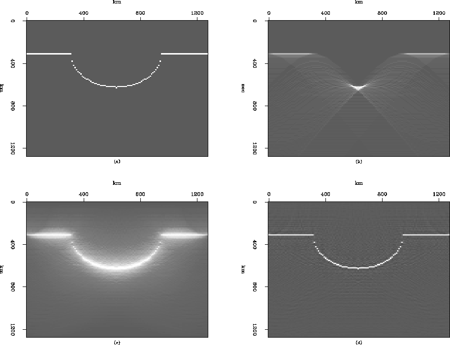
Figure ![[*]](http://sepwww.stanford.edu/latex2html/cross_ref_motif.gif) (a) shows a simple model with a syncline image.
The Kirchhoff modeling for the model [Figure
(a) shows a simple model with a syncline image.
The Kirchhoff modeling for the model [Figure ![[*]](http://sepwww.stanford.edu/latex2html/cross_ref_motif.gif) (a)]
is shown in Figure
(a)]
is shown in Figure ![[*]](http://sepwww.stanford.edu/latex2html/cross_ref_motif.gif) (b),
and the migration result is shown in Figure
(b),
and the migration result is shown in Figure ![[*]](http://sepwww.stanford.edu/latex2html/cross_ref_motif.gif) (c).
The image in Figure
(c).
The image in Figure ![[*]](http://sepwww.stanford.edu/latex2html/cross_ref_motif.gif) (c) is very blurred
compared to the original image.
We can suppress this artifact by the least-squares imaging;
the result is shown in Figure
(c) is very blurred
compared to the original image.
We can suppress this artifact by the least-squares imaging;
the result is shown in Figure ![[*]](http://sepwww.stanford.edu/latex2html/cross_ref_motif.gif) (d).
The image in Figure
(d).
The image in Figure ![[*]](http://sepwww.stanford.edu/latex2html/cross_ref_motif.gif) (d) is very close to the original image,
without any artifacts.
This result was obtained after only 5 iterations of the conjugate gradient
algorithm.
(d) is very close to the original image,
without any artifacts.
This result was obtained after only 5 iterations of the conjugate gradient
algorithm.
For more realistic synthetic model, I used Claerbout's synthetic model,
which has a very complicated geological model,
as shown in Figure ![[*]](http://sepwww.stanford.edu/latex2html/cross_ref_motif.gif) (a).
Figure
(a).
Figure ![[*]](http://sepwww.stanford.edu/latex2html/cross_ref_motif.gif) (b) shows the synthetic data generated
by the subroutine kirchfast(), and Figure
(b) shows the synthetic data generated
by the subroutine kirchfast(), and Figure ![[*]](http://sepwww.stanford.edu/latex2html/cross_ref_motif.gif) (c)
the result of migration.
The image after migration is smoother than the original image.
This suggests applying an
(c)
the result of migration.
The image after migration is smoother than the original image.
This suggests applying an  filter to recover the high frequency.
The image after the least-squares inversion, shown in
Figure
 ![[*]](http://sepwww.stanford.edu/latex2html/cross_ref_motif.gif) (d), contains more high frequency than the image
after migration.
The frequency recovery in the image after migration and inversion
is shown in Figure
(d), contains more high frequency than the image
after migration.
The frequency recovery in the image after migration and inversion
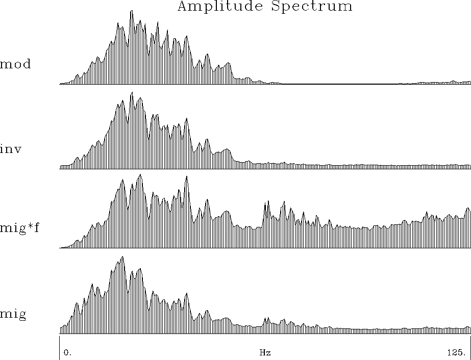
is shown in Figure ![[*]](http://sepwww.stanford.edu/latex2html/cross_ref_motif.gif) .
We can see that the spectrum of the image obtained
by the least-squares imaging is very close to the spectrum of the
original image.
Figure
.
We can see that the spectrum of the image obtained
by the least-squares imaging is very close to the spectrum of the
original image.
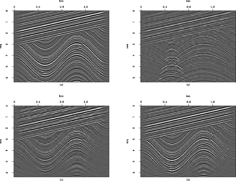
Figure ![[*]](http://sepwww.stanford.edu/latex2html/cross_ref_motif.gif) illustrates the same experiment as Figure
illustrates the same experiment as Figure ![[*]](http://sepwww.stanford.edu/latex2html/cross_ref_motif.gif) ,
except that the sampling interval is two times that of the sampling
interval of the model used in Figure
,
except that the sampling interval is two times that of the sampling
interval of the model used in Figure ![[*]](http://sepwww.stanford.edu/latex2html/cross_ref_motif.gif) .
The image after migration in Figure
.
The image after migration in Figure ![[*]](http://sepwww.stanford.edu/latex2html/cross_ref_motif.gif) (c) shows
artifacts because of the change in the sampling interval.
But the image obtained by the least-squares imaging,
Figure
(c) shows
artifacts because of the change in the sampling interval.
But the image obtained by the least-squares imaging,
Figure ![[*]](http://sepwww.stanford.edu/latex2html/cross_ref_motif.gif) (d), is still clear.
(d), is still clear.
Kirmiginv
Figure 1 Least-squares Kirchhoff imaging:
(a) Synthetic image model containing
a syncline reflector,
(b) Kirchhoff modeling,
(c) Kirchhoff migration for (b),
(d) Least-squares Kirchhoff imaging for (b)
(after 5 iterations of the conjugate gradient algorithm).
 kirinv3
Figure 2 Kirchhoff inversion:
(a) Synthetic image model with a syncline (nz=128 and nx=200),
(b) Kirchhoff modeling,
(c) Kirchhoff migration for (b),
(d) Least-squares Kirchhoff inversion for (b)
(after 10 iterations of the conjugate gradient algorithm).

kirspec3
Figure 3 Spectrum recovery after migration and inversion.
From the top: The spectrum of the original image,
of the inversed image, of the migration image times frequency,
and of the migration image.
|
|  |
 kirinv2
Figure 4 Kirchhoff inversion:
(a) Synthetic image model with a syncline (nz=128 and nx=100),
(b) Kirchhoff modeling,
(c) Kirchhoff migration for (b),
(d) Least-squares Kirchhoff inversion for (b)
(after 10 iterations of the conjugate gradient algorithm).

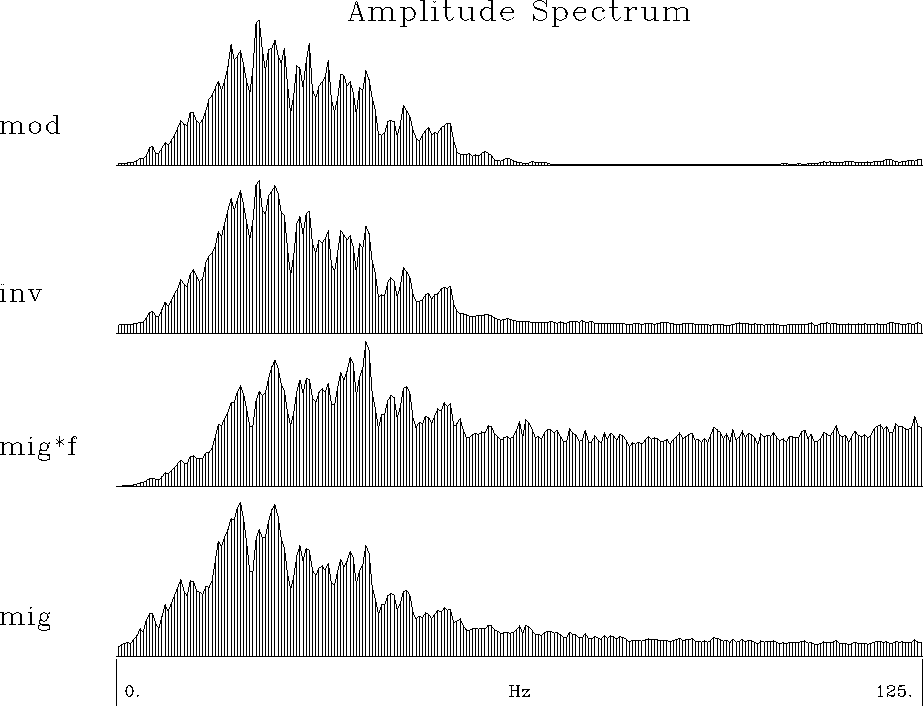
kirspec2
Figure 5 Spectrum recovery after migration and inversion.
From the top: The spectrum of the original image,
of the inversed image, of the migration image times frequency,
and of the migration image.
|
|  |


Next: Gazdag migration in v(z)
Up: LEAST-SQUARES IMAGING
Previous: LEAST-SQUARES IMAGING
Stanford Exploration Project
11/17/1997
![[*]](http://sepwww.stanford.edu/latex2html/cross_ref_motif.gif) (a).
Figure
(a).
Figure ![[*]](http://sepwww.stanford.edu/latex2html/cross_ref_motif.gif) (b) shows the synthetic data generated
by the subroutine kirchfast(), and Figure
(b) shows the synthetic data generated
by the subroutine kirchfast(), and Figure ![[*]](http://sepwww.stanford.edu/latex2html/cross_ref_motif.gif) (c)
the result of migration.
The image after migration is smoother than the original image.
This suggests applying an
(c)
the result of migration.
The image after migration is smoother than the original image.
This suggests applying an ![[*]](http://sepwww.stanford.edu/latex2html/cross_ref_motif.gif) (d), contains more high frequency than the image
after migration.
The frequency recovery in the image after migration and inversion
is shown in Figure
(d), contains more high frequency than the image
after migration.
The frequency recovery in the image after migration and inversion
is shown in Figure ![[*]](http://sepwww.stanford.edu/latex2html/cross_ref_motif.gif) .
We can see that the spectrum of the image obtained
by the least-squares imaging is very close to the spectrum of the
original image.
Figure
.
We can see that the spectrum of the image obtained
by the least-squares imaging is very close to the spectrum of the
original image.
Figure ![[*]](http://sepwww.stanford.edu/latex2html/cross_ref_motif.gif) illustrates the same experiment as Figure
illustrates the same experiment as Figure ![[*]](http://sepwww.stanford.edu/latex2html/cross_ref_motif.gif) ,
except that the sampling interval is two times that of the sampling
interval of the model used in Figure
,
except that the sampling interval is two times that of the sampling
interval of the model used in Figure ![[*]](http://sepwww.stanford.edu/latex2html/cross_ref_motif.gif) .
The image after migration in Figure
.
The image after migration in Figure ![[*]](http://sepwww.stanford.edu/latex2html/cross_ref_motif.gif) (c) shows
artifacts because of the change in the sampling interval.
But the image obtained by the least-squares imaging,
Figure
(c) shows
artifacts because of the change in the sampling interval.
But the image obtained by the least-squares imaging,
Figure ![[*]](http://sepwww.stanford.edu/latex2html/cross_ref_motif.gif) (d), is still clear.
(d), is still clear.
