

Next: CONCLUSIONS
Up: Michelena: Anisotropic tomography
Previous: SYNTHETIC EXAMPLE
In this section, I show the application of the technique previously
explained to a cross-well data set recorded at BP's Devine test site,
located southwest of San Antonio, Texas.
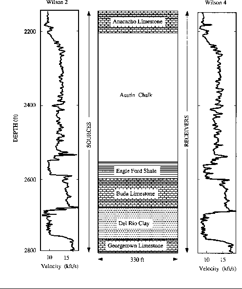
A sketch of the geology at this site is shown in Figure ![[*]](http://sepwww.stanford.edu/latex2html/cross_ref_motif.gif) .
This test site has been cited in recent
publications to illustrate the application
of different techniques.
For example,
Harris (1988) reports cross-well seismic measurements using a
cylindrical piezoelectric bender transducer both
as a source and as a receiver.
Miller and Chapman (1991) and Onishi and Harris (1991)
concentrate on the problem of estimating
velocity anisotropy from cross-well data (tomographically and by
head-wave analysis, respectively). Lazaratos et al. (1991) present
reflection images also
from the cross-well data and Raikes (1991)
studies the propagation of S-waves from a multicomponent VSP.
.
This test site has been cited in recent
publications to illustrate the application
of different techniques.
For example,
Harris (1988) reports cross-well seismic measurements using a
cylindrical piezoelectric bender transducer both
as a source and as a receiver.
Miller and Chapman (1991) and Onishi and Harris (1991)
concentrate on the problem of estimating
velocity anisotropy from cross-well data (tomographically and by
head-wave analysis, respectively). Lazaratos et al. (1991) present
reflection images also
from the cross-well data and Raikes (1991)
studies the propagation of S-waves from a multicomponent VSP.
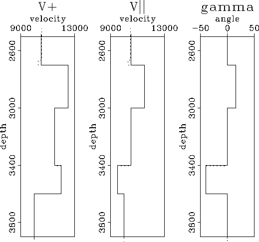
final-model-profile-syn
Figure 7 Profile at x=0 of the real model and the
estimated one (Figures 4 and 7 respectively).
The continuos line represents the
real model and the dashed one the result of the inversion. The agreement
between real and estimated parameters
is almost perfect.
``V+'' stands for  ,``V||'' for
  and ``gamma'' for
  .
.

The cross-well data I will use in this paper are
P-waves with frequencies between
200 Hz and 4000 Hz. They were recorded between two cased boreholes
(Wilson 2 and Wilson 4) whose
separation at the surface was 330 ft. Receivers
were separated 10 ft and sources 20 ft. Figure ![[*]](http://sepwww.stanford.edu/latex2html/cross_ref_motif.gif) shows
the corresponding
sonic logs at each well. Although the variations are mainly
1-D,
it is possible
to identify from the logs small dips (
shows
the corresponding
sonic logs at each well. Although the variations are mainly
1-D,
it is possible
to identify from the logs small dips ( 1 degree)
from one well to the other as well as small lateral variations within thin
layers (for example, the top of
the Del Rio clay).
1660 traveltimes were picked from a small data set of only 26 gathers.
From these traveltimes only those corresponding
to angles less than 45 degrees between source and receiver were
kept for the inversion.
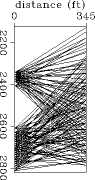
Figure ![[*]](http://sepwww.stanford.edu/latex2html/cross_ref_motif.gif) shows positions of sources and receivers
for 10% of the data set. Notice how irregular the ray coverage
is specially in terms of horizontal rays, not present in large portions
of the medium.
The horizontal velocities estimated in those
areas, unlike the rest of the medium,
will be the horizontal NMO
velocities, that is, horizontal velocities of the best fitting ellipses.
shows positions of sources and receivers
for 10% of the data set. Notice how irregular the ray coverage
is specially in terms of horizontal rays, not present in large portions
of the medium.
The horizontal velocities estimated in those
areas, unlike the rest of the medium,
will be the horizontal NMO
velocities, that is, horizontal velocities of the best fitting ellipses.
The starting model
(not shown) consisted of 140 horizontal layers
5 ft thick. The velocity for all layers was 12000 ft/sec. Layers thinner
than 1 ft were not allowed in the model.
The inversion was not constrained to match
the vertical velocities or
depth of certain layers using information derived from
the sonic logs, although the information of dips is already
present in the initial model.
devine-site
Figure 8 Sketch of the geology at the Devine test site
with the sonic logs at each well. Although
mostly flat layered, small 2-D variations can be seen (modified from
Lazaratos et al., (1991).
 devine-rays
Figure 9 Ray coverage for the experiment at the Devine test site for a
fraction (10%) of the total data set. Notice how irregular
the coverage is.

The inversion produced a model with horizontal layers (all
dips less than 0.1 degree) and vertical axes of symmetry. Therefore,
 and
and  .Figure
 ![[*]](http://sepwww.stanford.edu/latex2html/cross_ref_motif.gif) shows
the horizontal and vertical velocities
as well
as an average sonic log from the two wells, blocked every 7 ft.
The first thing we notice from Figure
shows
the horizontal and vertical velocities
as well
as an average sonic log from the two wells, blocked every 7 ft.
The first thing we notice from Figure ![[*]](http://sepwww.stanford.edu/latex2html/cross_ref_motif.gif) is that
is that  for almost all depths. We also notice that
Vz is much closer to the sonic log than Vx, which is
more than 30% larger than the log velocity in the shale and
clay intervals.
The vertical velocity contrast between limestone and shale
is greater than 70%. Still,
the inversion does a good job in estimating Vz.
For this model,
the average absolute value of the residuals is 0.2 ms (twice the sampling
interval).
12 layers were eliminated during the inversion procedure.
These results agree with the ones presented by Miller and Chapman (1991)
and Onishi and Harris (1991).
Figure ![[*]](http://sepwww.stanford.edu/latex2html/cross_ref_motif.gif) also shows that
the elliptical
velocity model explains most of
the P-wave anisotropy at this site. However,
note that the estimated
vertical velocity (NMO velocity) is in general smaller than the log velocity,
which indicates that the elliptical model is not fully adequate to describe
the possible transverse isotropic nature of this medium.
In a few places
(top of the clay, for example)
the estimated vertical velocities are
larger than the log velocity. This is probably
because of lateral variations in the real medium
that are
not correctly described by the model of heterogeneities.
also shows that
the elliptical
velocity model explains most of
the P-wave anisotropy at this site. However,
note that the estimated
vertical velocity (NMO velocity) is in general smaller than the log velocity,
which indicates that the elliptical model is not fully adequate to describe
the possible transverse isotropic nature of this medium.
In a few places
(top of the clay, for example)
the estimated vertical velocities are
larger than the log velocity. This is probably
because of lateral variations in the real medium
that are
not correctly described by the model of heterogeneities.
In order to better characterize
the nature of the anisotropy, additional wave types
and measurement directions (from a VSP survey for example) are
needed.


Next: CONCLUSIONS
Up: Michelena: Anisotropic tomography
Previous: SYNTHETIC EXAMPLE
Stanford Exploration Project
11/18/1997
![[*]](http://sepwww.stanford.edu/latex2html/cross_ref_motif.gif) .
This test site has been cited in recent
publications to illustrate the application
of different techniques.
For example,
Harris (1988) reports cross-well seismic measurements using a
cylindrical piezoelectric bender transducer both
as a source and as a receiver.
Miller and Chapman (1991) and Onishi and Harris (1991)
concentrate on the problem of estimating
velocity anisotropy from cross-well data (tomographically and by
head-wave analysis, respectively). Lazaratos et al. (1991) present
reflection images also
from the cross-well data and Raikes (1991)
studies the propagation of S-waves from a multicomponent VSP.
.
This test site has been cited in recent
publications to illustrate the application
of different techniques.
For example,
Harris (1988) reports cross-well seismic measurements using a
cylindrical piezoelectric bender transducer both
as a source and as a receiver.
Miller and Chapman (1991) and Onishi and Harris (1991)
concentrate on the problem of estimating
velocity anisotropy from cross-well data (tomographically and by
head-wave analysis, respectively). Lazaratos et al. (1991) present
reflection images also
from the cross-well data and Raikes (1991)
studies the propagation of S-waves from a multicomponent VSP.


