Next: INVERSE MODELING
Up: Michelena: Anisotropic tomography
Previous: Introduction
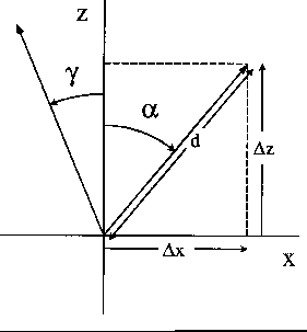
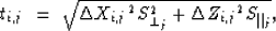
The traveltime for a ray that travels a distance d in an
homogeneous medium with
elliptical anisotropy and axis of symmetry forming an angle  with respect to the vertical (Figure
 ![[*]](http://sepwww.stanford.edu/latex2html/cross_ref_motif.gif) ) is
) is
| 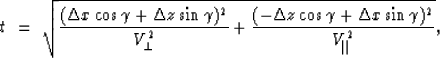 |
(1) |
where 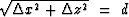 and
and  and
and
 are the velocities in the directions parallel and perpendicular
respectively
to the axis of symmetry. In Appendix A, I explain how to
derive this expression.
ray-and-axis
are the velocities in the directions parallel and perpendicular
respectively
to the axis of symmetry. In Appendix A, I explain how to
derive this expression.
ray-and-axis
Figure 1 Ray traveling a distance d in a medium with tilted
axis of symmetry.  and are the angles of the
ray and the axis of symmetry respectively with respect to the vertical.
and are the angles of the
ray and the axis of symmetry respectively with respect to the vertical.

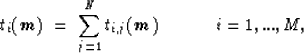
If the model is described as a superposition of N homogeneous orthogonal
regions, the traveltime for the ith ray traveling across
the jth region is
| 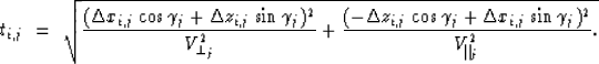 |
(2) |
Note that each homogeneous region is
characterized by three parameters: two velocities and the angle of the
axis of symmetry with respect to the vertical. From now on
I will refer to this parameters as interval parameters. In the previous
equation, 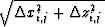 is the distance
traveled by the ith ray in the jth cell.
The sum of expressions
like equation
(2) can be used to compute the traveltime from source to receiver
for a ray that travels in an heterogeneous media, assuming the ray
path is known. Byun (1982) and Michelena (1992)
explain how to do the ray tracing.
is the distance
traveled by the ith ray in the jth cell.
The sum of expressions
like equation
(2) can be used to compute the traveltime from source to receiver
for a ray that travels in an heterogeneous media, assuming the ray
path is known. Byun (1982) and Michelena (1992)
explain how to do the ray tracing.
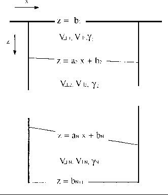
Figure shows the type of model that I will
consider in this paper.
It consists of
homogeneous elliptically
anisotropic
blocks separated by straight
interfaces of variable dip (aj) and intercept (bj).
I assume that all the axes
of symmetry for the different layers lie in the same plane
of the survey geometry.
If  and
and  are defined as
|  |
(1) |
| (2) |
the expression (2) for the traveltime ti,j
of the ith ray in the jth cell becomes
|  |
(4) |
where
 ,
,  ,
,  and
and
 are equal to


(xi,j, zi,j) is the point of intersection
between the
ith ray and the jth interface.
If the axis of symmetry is vertical
( ), it follows that
 and
and  .
inv-model
.
inv-model
Figure 2 Model of velocities and heterogeneities. The top and bottom interfaces
are horizontal (a1 = aN+1 = 0) and located at known depths.
Besides the interval parameters previously described,
I have added two more parameters
to describe how the boundaries that separate different intervals
may change their
positions. I call these parameters boundary parameters.
Figure shows how to count both intervals and
boundaries.
The total traveltime for a ray that travels from source to receiver is
|  |
(5) |
where  is the vector of model parameters of
5N elements:
is the vector of model parameters of
5N elements:
|  |
|
| (6) |
and M is the total number of traveltimes.
Equation (5) is the system of nonlinear equations that relates the model
parameters with the measured traveltimes. A linearized version
of this equations will be used in the next section
to solve the inverse problem. As explained in Figure ,
b1 and a1 are known. This
makes the number of variables in equal
to 5N - 2.
Next: INVERSE MODELING
Up: Michelena: Anisotropic tomography
Previous: Introduction
Stanford Exploration Project
11/18/1997