|
hyp
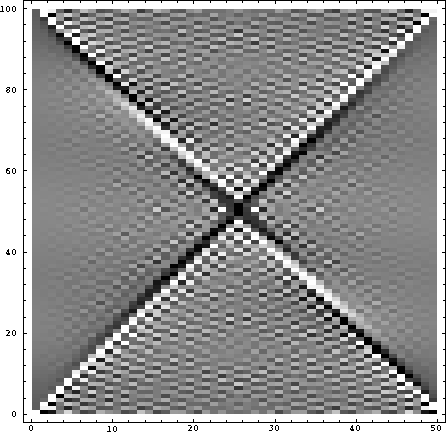
Figure 1 The original hyperbola with constant amplitude sample values. |  |
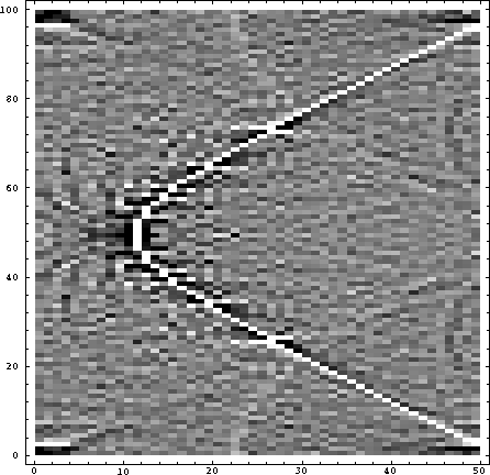
As a comparison between developing a process using Mathematica and using the standard SEP software, hyperbola whitening is considered. Here, a hyperbola is generated with constant amplitude at each sample. The hyperbola is whitened by transforming the matrix containing it with a two-dimensional Fourier transform, dividing the transformed data by its absolute value, and inverse transforming back to the original domain. The new hyperbola will have a amplitude different from the original hyperbola. Using Mathematica, the process is implemented as follows:
v=6000.
t0=0.05
n1=100
n2=50
xinc = 25.0
tinc = 0.004
          (* create an empty matrix *)
data = Table[N[0.],{i,1,n1},{j,1,n2}];
          (* build a hyperbola within the matrix *)
For[i=1, i<n1+1,i ++, x=(i-n1/2) xinc; t=Sqrt[(x^2/(v^2) + t0^2)]; j= Floor[t/
tinc];data[[i,j]] = N[1.0] ]
          (* display the hyperbola *)
ListDensityPlot[data,Mesh->False]
          (* do a 2-D Fourier transform *)
fdata =Fourier[data];
ListDensityPlot[Re[fdata],Mesh->False]
          (* divide the transformed data by its absolute value *)
sdata = fdata/Abs[fdata];
newdata = InverseFourier[sdata];
          (* display the final result  *)
ListDensityPlot[Re[newdata],Mesh->False]
Notice that the matrix `fdata' does not have to be dimensioned or specified as an array of complex numbers. However, note that the final display of `newdata' plotted only the real part of the matrix, since the ListDensityPlot routine expects real numbers. ListDensityPlot produces a raster-like display using various gray-scale densities. The `Mesh->False' option removes the default overlay mesh that generally obliterates seismic data. The Fourier routine applies a Fourier transform to an object supplied to it. If the object has two dimensions, such as our matrix, it will do a two-dimensional Fourier transform. To apply a Fourier transform to only one axis of a matrix, use Map[Fourier,a]. The expression `fdata/Abs[fdata]' divides each element of the complex matrix fdata by the absolute value of the corresponding element. The actual matrix multiplication and matrix inversion are done with different syntax.
The three displays created by this run are shown in Figures 1 to 3.
|
hyp
Figure 1 The original hyperbola with constant amplitude sample values. |  |
|
hypfk
Figure 2 The real part of the Fourier transform of the original hyperbola. |  |
|
newhyp
Figure 3 The hyperbola created from the inverse Fourier transform of the scaled data. |  |
The comparable run using standard SEP software is as follows:
Spike n1=50 n2=100 k1=10 >spike.H
~/fort/hyper <spike.H >hyper.H
Bandpass <hyper.H >filter.H fhi=100
Rtoc <filter.H >cfilter.H
Ft3d sign1=1 sign2=1 <cfilter.H >cfft.H
Real <cfft.H >rfft.H
Cabs <cfft.H >absfft.H
Rtoc <absfft.H >cabsfft.H
Real <cfft.H >rjunk.H
Imag <cfft.H >ijunk.H
Add  rjunk.H absfft.H mode=d > rdjunk.H
Add  ijunk.H absfft.H mode=d > idjunk.H
Cmplx rdjunk.H idjunk.H >dfft.H
Rm *unk.H
Ft3d sign1=-1 sign2=-1 <dfft.H >cdinvfft.H
Real <cdinvfft.H >invfft.H
Taplot <invfft.H|Ta2vplot|Tube
Taplot < filter.H  | Ta2vplot | Tube
Taplot <rfft.H|Ta2vplot|Tube
The only nonstandard routine used here is the hyper routine that corresponds to the first ten lines of the Mathematica code. It is used to replace the spike synthetic with a hyperbola and is not shown here.
For small processes like this one, where the run time is insignificant compared to the coding time, Mathematica provides a quick method of getting results. For runs with significantly longer run times or for larger datasets, the standard SEP software is preferable since it is not limited to the memory size of the machine being used. The SEP software will run faster in computationally intense jobs, where Mathematica would be inpractical because of the overhead associated with the extra flexibility provided. Mathematica's interactive mode does provide more flexibility for observing the intermediate results than do the traditional FORTRAN or C codes.
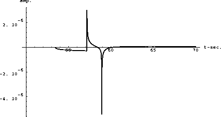
A second sample shows a job building a Cagniard-De Hoop impulse response. The expression for the impulse response is shown here as given in Aki and Richards(1980).
| (1) |
| (2) |
| (3) |
Coding and debugging these equations in FORTRAN or C would take some time, especially since several variables in the above equations are dependent on other variables, as seen below. The Mathematica input corresponding to these equations is as follows:
(* define a Heaviside function *)
H[xtemp_Real] :=
   ytemp = If[xtemp >= 0., 1., 0. ];Return[ytemp]

(* Set up the Cagniard-De Hoop equations *)

c = A/(2 Pi rho1 beta1^2)
c2 = (mu1 eta1 - mu2 eta2)/(mu1 eta1 + mu2 eta2)
refl = c Im[c2] (H[t-tn] - H[t-R0/beta1])/Sqrt[R0^2/beta1^2 - t^2]
refr = c Re[c2] (H[t-R0/beta1])/Sqrt[-R0^2/beta1^2 + t^2]
dirt = A/(2 Pi rho1 beta1^2) H[t-x/beta1]/( (t^2 - x^2/beta1^2)^(1/2) )

(*  fill in the variables *)
mu1 = beta1^2 rho1
mu2 = beta2^2 rho2
R0 = (x^2 + (z+z0)^2)^(1/2)
eta1 = (1/( beta1^2 ) - p^2)^(1/2)
eta2 = (1/( beta2^2 ) - p^2)^(1/2)
tn = x/beta2 + Abs[z+z0] (1/beta1^2 - 1/beta2^2)^(1/2)
p = ( x t + I Abs[z+z0] (t^2 - R0^2/beta1^2)^(1/2) )/( R0^2)

(* now define the actual values *)
beta1 = 3.5
rho1 = 2700
beta2 = 4.5
rho2 = 3300
x = 200
z0 = 25
z = 25
A = 1.

(* put the direct, reflected, and refracted arrivals together *)
all = dirt + refl + refr

(* Plot it *)
axx = Re[all]
plot = Plot[axx,{t,50,70},PlotRange->All,AxesLabel->{"t-sec.","amp."}]
A FORTRAN program is likely to be similar, except that the first few blocks of code would be reversed. With Mathematica, each expression may be printed as the variables are filled in, allowing the intermediate expressions to be examined to save debugging time. The standard Plot routine is used to display the output shown in figure 4.
 |