SEISMIC DATA EXAMPLES

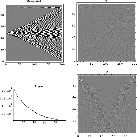
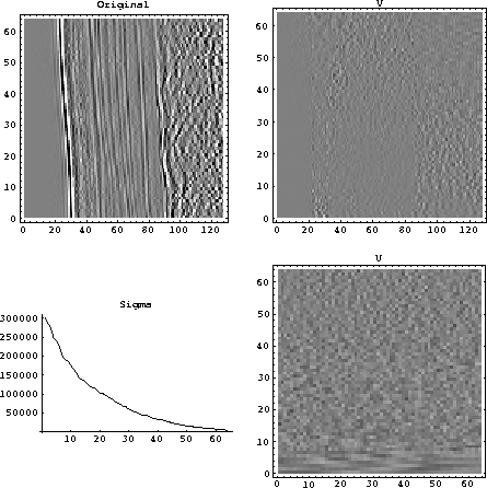
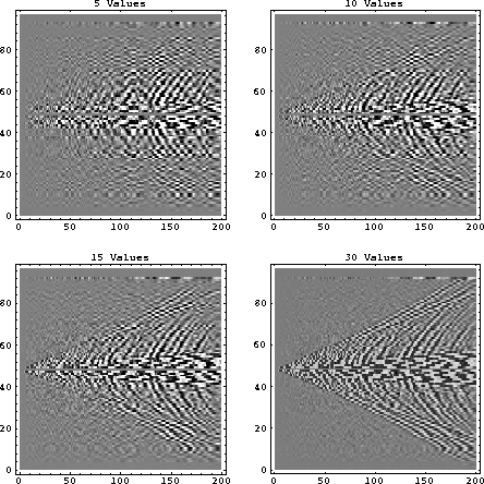
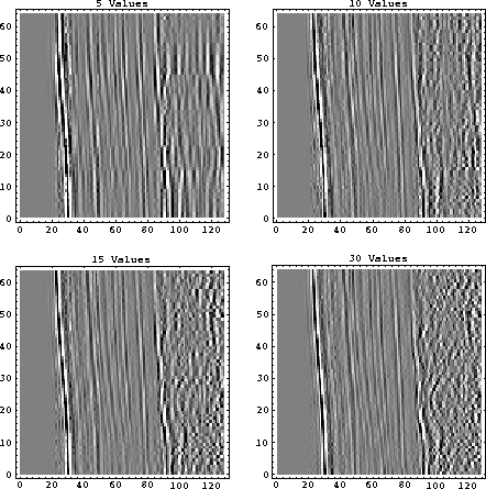
The first example of decomposing a seismic record is the shot record shown in Figure 8. The plot of $\Sigma$ shown in the figure shows the singular values decreasing slowly compared to the those in the photographic case. The U matrix also shows significant detail on the vectors corresponding to the smaller singular values. The reconstructions of the shot gather using a only few of the larger singular values are shown in Figure 9. When only five singular values are used to reconstruct the shot gather, much of the dipping energy is lost, but as more singular values are used, the steeper dips gradually reappear. Even while using 30 singular values, the shot gather is poorly reconstructed. Most of the high amplitude events have reappeared, but the small details are washed out, and noise has corrupted the low amplitude background above the first breaks.

 

shotsvd
Figure 8 A shot gather and its decomposition. Notice the slow decrease in the size of the singular values and the structure evident in the U matrix.

 

shotreci
Figure 9 The shot gather reconstructed using 5, 10, 15, and 30 singular values. Events with low dips are reconstructed with the first few singular values, and the higher dips appear with the smaller singular values added later.

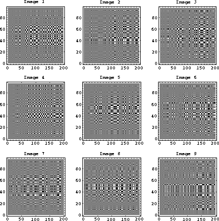
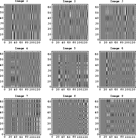
Figure 10 has been included here to give the reader an idea of what the images corresponding to the first few singular values of the shot gather look like. Here vertical and horizontal patterns make it obvious that the images are the outer products of two vectors. The first few images in Figure 10 have the energy concentrated about the central portion of the image. This corresponds roughly to the reconstructions shown in Figure 9, where the flat data in the center is reconstructed first. The steep-dip data in the outer traces associated with the smaller singular values are imaged with the later, smaller singular values.

 

shotiter
Figure 10 The images of a shot gather associated with the first nine singular values. Here it becomes obvious that the images are constructed from the outer product of two vectors.

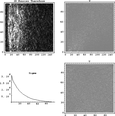
In an attempt to simplify the input to the singular value decomposition, a two-dimensional Fourier transform was applied to the shot record. The transform, as seen in Figure 11, shows that much of the energy is concentrated in the lower frequency range. While dips are still present, the dips are smaller than those in the original shot gather. It is interesting to see that the plot of the singular values appears to be similar to the plot of the singular values of the original shot gather shown in Figure 8. Although much of the detail in the U and V matrices is lost because the plots show the absolute value of the complex numbers, the U and V matrices appear much simpler than the U and V matrices of the original shot gathers.

 

2dfftsvd
Figure 11 The two-D Fourier transform of the shot gather and its decomposition. Notice the slow decrease in the size of the singular values and compare these singular values to the singular values shown in Figure 8.

More success compressing stacked datasets is expected, since these data contain fewer high-amplitude steep-dip events than typical shot gathers. The stack shown in Figure 12 contains gently sloping events below the water bottom and more complex structures deeper in the section. The plot of the singular values shows a pattern similar to the singular values of the shot gather, which is surprising, since the dips are smaller and the dipping events are of lower amplitude in the stacked case. When the original data is reconstructed from the stack's decomposition using the first few singular values, discontinuities can be seen in the first few reconstructions shown in Figure 13. The steeper dips missing on the first few reconstructions do not appear until the last reconstruction using 30 singular values.

 

stksvd
Figure 12 A stack and it's decomposition. While the stack appears simpler than the shot gather shown in Figure 8, the slow decrease of the singular values is similar.

 

stackreci
Figure 13 The stack reconstructed using 5, 10, 15, and 30 singular values. Notice the discontinuities in the shallow zone and the lost diffraction tails in the deeper zone for the reconstructions using 5 and 10 values.

Figure 14 shows the images associated with the first few singular values and gives some insight into the discontinuities seen in the reconstructions shown in Figure 13. The reflections are broken up into events consisting of alternating polarities with spatial periods that generally decrease as the size of the singular values decrease. As more singular values are used, more detail is seen in the reconstruction.

 

stkiter
Figure 14 The stack images associated with the first nine singular values.

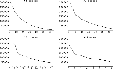
While it might be hoped that increasing or decreasing the number of traces put into the singular value decomposition might change the trend of the singular values, this effect is not seen with the stack image. Figure 15 shows the singular values for various numbers of traces from the stack in Figure 12. The slow decrease in amplitude of the singular values is similar for all these cases.

 

stackvar
Figure 15 Sizes of the singular values using 64, 32, 16, and 8 traces of a stack image. The slow decrease in amplitude is similar for these cases.