Next: Conclusions
Up: Karrenbach: source equalization
Previous: The Pembrook data set
The optimization problems described by E1 and E2 were solved using
a conjugate gradient method. I chose to constrain the first filter in each of
the series of filters to unity. Thus I chose the first shot
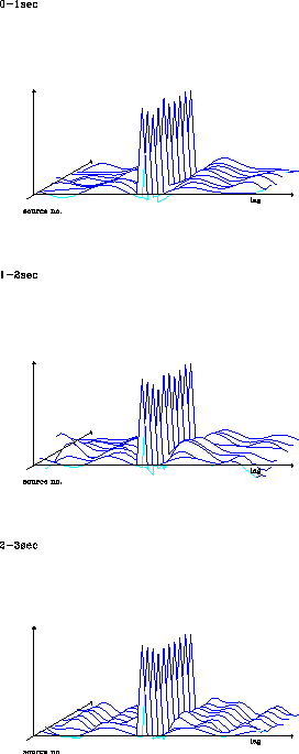
gather to be my reference gather. Figure ![[*]](http://sepwww.stanford.edu/latex2html/cross_ref_motif.gif) and show results
obtained during testing the nonstationarity of the recorded data
on a few shot gathers.
I tried different window sizes and shapes, but the answers, after about 40
iterations, were always very similar to and .
This behavior encouraged me to apply the equalization process about 50
shotgathers in a two second time window, knowing that this time window
averages over a fair amount of energy that is radiated from the source
with different emergence angles.
I chose to use a medium length filter of about 40 points (160 msec).
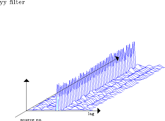
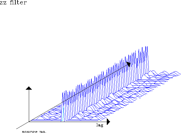
Results of those equalizations are shown in two groups. First a minimization
described by E2 for the components Xx, Yy and Zz
(capital letters denote source components,
lower-case letters denote receiver components).
The prediction
error filters obtained are shown in Figures , and
. The filter obtained after about 40 iterations is minimum
phase. There seem to be hardly any time shifts between different source
points. The amplitude in the main peak and lower energy wavelet characterize
all the filters consistently.
Figure shows a comparison between the raw prestack time slice
and the filtered version. The differences in that time slice are small
but noticeable. The continuity in character of the time slice is increased.
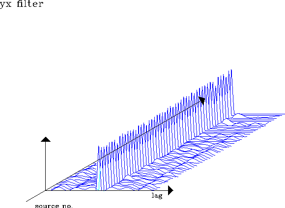
Figures to are obtained from maximizing symmetry
in the prestack data using the objective function E1, where all components
are equalized simultaneously. The offdiagonal elements in the three-by-three
filter set show identical behavior. Again the filter are consistent along
the line and exhibit the similar properties as the filters in Figures
to .
The short 1-D filters equalize by averaging over an angular distribution of
radiation pattern. The amount of averaging is determined by the time window
and number of different arrivals within the time window.
and show results
obtained during testing the nonstationarity of the recorded data
on a few shot gathers.
I tried different window sizes and shapes, but the answers, after about 40
iterations, were always very similar to and .
This behavior encouraged me to apply the equalization process about 50
shotgathers in a two second time window, knowing that this time window
averages over a fair amount of energy that is radiated from the source
with different emergence angles.
I chose to use a medium length filter of about 40 points (160 msec).
Results of those equalizations are shown in two groups. First a minimization
described by E2 for the components Xx, Yy and Zz
(capital letters denote source components,
lower-case letters denote receiver components).
The prediction
error filters obtained are shown in Figures , and
. The filter obtained after about 40 iterations is minimum
phase. There seem to be hardly any time shifts between different source
points. The amplitude in the main peak and lower energy wavelet characterize
all the filters consistently.
Figure shows a comparison between the raw prestack time slice
and the filtered version. The differences in that time slice are small
but noticeable. The continuity in character of the time slice is increased.
Figures to are obtained from maximizing symmetry
in the prestack data using the objective function E1, where all components
are equalized simultaneously. The offdiagonal elements in the three-by-three
filter set show identical behavior. Again the filter are consistent along
the line and exhibit the similar properties as the filters in Figures
to .
The short 1-D filters equalize by averaging over an angular distribution of
radiation pattern. The amount of averaging is determined by the time window
and number of different arrivals within the time window.
In the future I plan to investigate how strong the influence of such an
equalization is on the results produced by a simple stack, velocity
analysis and migration, thus determining when it is necessary to estimate
the radiation pattern in an absolute manner instead of, as shown here, a
purely relative manner.
fig1
Figure 7 Prediction error filters at 10 locations
estimated from 0-3 seconds in one-second-long windows of the data.


 fig2
fig2
Figure 8 Prediction error filters at 10 locations
estimated from 3-7 seconds in one-second-long windows of the data.
filsxx
Figure 9 Prediction error filters at 50 locations
estimated for X source component and x receiver component in a two-second-time window. Minimizes objective function E2.
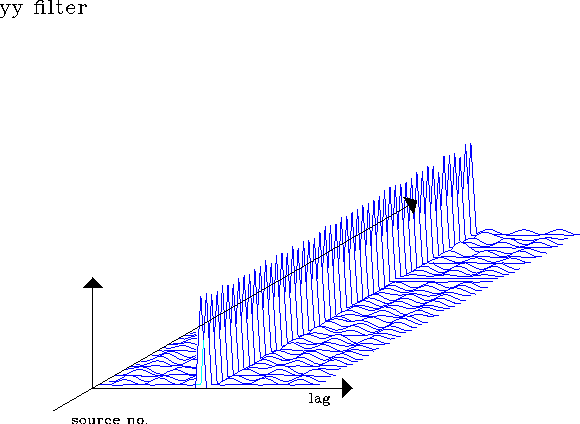
filsyy
Figure 10 Prediction error filters at 50 locations
estimated for Y source component and y receiver component in a two-second-time window. Minimizes objective function E2.
filszz
Figure 11 Prediction error filters at 50 locations
estimated for Z source component and z receiver component in a two-second-time window. Minimizes objective function E2.
compxx
Figure 12 Raw and equalized time slice of the part of the data for which reciprocal data exist for 50 source points (Xx-component). To go through time slices, press the button.
filxx.40
Figure 13 Prediction error filters at 50 locations
estimated for X source component and x receiver component in a two-second-time window. Minimizes objective function E1.
filxy.40
Figure 14 Prediction error filters at 50 locations
estimated for X source component and y receiver component in a two-second-time window. Minimizes objective function E1.
filxz.40
Figure 15 Prediction error filters at 50 locations
estimated for X source component and z receiver component in a two-second-time window. Minimizes objective function E1.
filyx.40
Figure 16 Prediction error filters at 50 locations
estimated for Y source component and x receiver component in a two-second-time window. Minimizes objective function E1.
filyy.40
Figure 17 Prediction error filters at 50 locations
estimated for Y source component and y receiver component in a two-second-time window. Minimizes objective function E1.
filyz.40
Figure 18 Prediction error filters at 50 locations
estimated for Y source component and z receiver component in a two-second-time window. Minimizes objective function E1.
filzx.40
Figure 19 Prediction error filters at 50 locations
estimated for Z source component and x receiver component in a two-second-time window. Minimizes objective function E1.
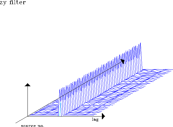
filzy.40
Figure 20 Prediction error filters at 50 locations
estimated for Z source component and y receiver component in a two-second-time window. Minimizes objective function E1.
filzz.40
Figure 21 Prediction error filters at 50 locations
estimated for Z source component and z receiver component in a two-second-time window. Minimizes objective function E1.
Next: Conclusions
Up: Karrenbach: source equalization
Previous: The Pembrook data set
Stanford Exploration Project
11/18/1997