

Next: Summary of the algorithm
Up: DEALIASING THE PREDICTION FILTERS
Previous: The zeros of prediction
Dealiasing the prediction filter  is a process of identifying,
for each frequency, L of its zeros that are also zeros of the prediction
filter
  . Let us call these L zeros of
  ``genuine'' zeros and the rest (M-1)L zeros ``fake'' zeros.
Comparing equations (13) with (11) shows
that, for genuine zeros,
  in equation (13)
vanishes; while for fake zeros,
  does not vanish.
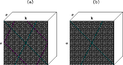
Hence, if we project all zeros of
  onto the
  -kx
plane, as shown in Figure
 ![[*]](http://sepwww.stanford.edu/latex2html/cross_ref_motif.gif) , the location of each genuine
zero as the function of
, the location of each genuine
zero as the function of  follows a linear trajectory which, or
the extension of which, passes through the origin. The location of each fake
zero also follows a linear trajectory, but neither this trajectory nor
its extension passes the origin. Equation (13) also shows
we know that each genuine zero has (M-1) fake zeros associated
with it. We can predict where the associated fake zeros are if
we know the position of the genuine zero. From above observations,
it is apparent that dealiasing the prediction filter is equivalent to a pattern
recognition process that retains the genuine zeros and rejects
fake zeros. Our method uses a neural net to accomplish this goal.
zind
Figure 1 The principle of dealiasing the prediction filter. Each black dot indicates
the projection of a zero of the prediction filter onto the  -k plane:
(a) before dealiasing; (b) after dealiasing.


To design a neural net for the problem, we must first find all zeros of the
prediction filter  by scanning the spectrum of the filter
over the s plane. Then we project these zeros onto the
discretized
  -kx plane. We define the input
zero-indicator array as follows:
|  |
(14) |
and, similarly, the output zero-indicator array is defined as follows:
|  |
(15) |
Now we can retain a genuine zero by setting its indicator to 1 and
reject a fake zero by setting its indicator to .
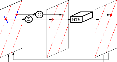
For each vij=1, we define two regions, the exhibition region Cij
and the inhibition region Dij. The exhibition region contains the
indicators that are on the linear trajectory passing
through both position (i,j)
and the origin, and that are in the neighborhood of position (i,j).
The inhibition region contains the indicators that indicate the associated
fake zeros. Next, we compute
|  |
(16) |
where |Cij| is the number of indicators in Cij. Then we use
the winner-take-all (WTA) algorithm to determine the value of uij,
as follows:
|  |
(17) |
This algorithm is applied iteratively, as shown in Figure ![[*]](http://sepwww.stanford.edu/latex2html/cross_ref_motif.gif) .
Figure
.
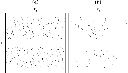
Figure ![[*]](http://sepwww.stanford.edu/latex2html/cross_ref_motif.gif) displays an example of dealiasing the zeros of the
prediction filters computed from field data. In spite of a few mistakes
that can be identified by the human eye, the result is satisfactory.
Most of the genuine zeros are retained and the fake zeros removed.
Noted that the convergence of the iterative WTA algorithm
is not guaranteed. However, the algorithm will never diverge because of
the discrete and finite nature of the problem. Generally speaking,
after several iterations, the output of the algorithm will oscillate
among a few solutions that are all close to the globally optimal solution.
neunet2
displays an example of dealiasing the zeros of the
prediction filters computed from field data. In spite of a few mistakes
that can be identified by the human eye, the result is satisfactory.
Most of the genuine zeros are retained and the fake zeros removed.
Noted that the convergence of the iterative WTA algorithm
is not guaranteed. However, the algorithm will never diverge because of
the discrete and finite nature of the problem. Generally speaking,
after several iterations, the output of the algorithm will oscillate
among a few solutions that are all close to the globally optimal solution.
neunet2
Figure 2 An illustration of the iterative winner-take-all (WTA) algorithm.
 cwlneu
Figure 3 An example of dealiasing the prediction filter with a neural net:
(a) input zero indicators, (b) output zero indicators.


Next: Summary of the algorithm
Up: DEALIASING THE PREDICTION FILTERS
Previous: The zeros of prediction
Stanford Exploration Project
11/18/1997
![[*]](http://sepwww.stanford.edu/latex2html/cross_ref_motif.gif) , the location of each genuine
zero as the function of
, the location of each genuine
zero as the function of ![]() is a process of identifying,
for each frequency, L of its zeros that are also zeros of the prediction
filter
is a process of identifying,
for each frequency, L of its zeros that are also zeros of the prediction
filter ![]() . Let us call these L zeros of
. Let us call these L zeros of ![]() ``genuine'' zeros and the rest (M-1)L zeros ``fake'' zeros.
Comparing equations (13) with (11) shows
that, for genuine zeros,
``genuine'' zeros and the rest (M-1)L zeros ``fake'' zeros.
Comparing equations (13) with (11) shows
that, for genuine zeros, ![]() in equation (13)
vanishes; while for fake zeros,
in equation (13)
vanishes; while for fake zeros, ![]() does not vanish.
Hence, if we project all zeros of
does not vanish.
Hence, if we project all zeros of ![]() onto the
onto the ![]() -kx
plane, as shown in Figure
-kx
plane, as shown in Figure ![[*]](http://sepwww.stanford.edu/latex2html/cross_ref_motif.gif) , the location of each genuine
zero as the function of
, the location of each genuine
zero as the function of ![]() follows a linear trajectory which, or
the extension of which, passes through the origin. The location of each fake
zero also follows a linear trajectory, but neither this trajectory nor
its extension passes the origin. Equation (13) also shows
we know that each genuine zero has (M-1) fake zeros associated
with it. We can predict where the associated fake zeros are if
we know the position of the genuine zero. From above observations,
it is apparent that dealiasing the prediction filter is equivalent to a pattern
recognition process that retains the genuine zeros and rejects
fake zeros. Our method uses a neural net to accomplish this goal.
follows a linear trajectory which, or
the extension of which, passes through the origin. The location of each fake
zero also follows a linear trajectory, but neither this trajectory nor
its extension passes the origin. Equation (13) also shows
we know that each genuine zero has (M-1) fake zeros associated
with it. We can predict where the associated fake zeros are if
we know the position of the genuine zero. From above observations,
it is apparent that dealiasing the prediction filter is equivalent to a pattern
recognition process that retains the genuine zeros and rejects
fake zeros. Our method uses a neural net to accomplish this goal.

![]() by scanning the spectrum of the filter
over the s plane. Then we project these zeros onto the
discretized
by scanning the spectrum of the filter
over the s plane. Then we project these zeros onto the
discretized ![]() -kx plane. We define the input
zero-indicator array as follows:
-kx plane. We define the input
zero-indicator array as follows:


![[*]](http://sepwww.stanford.edu/latex2html/cross_ref_motif.gif) .
Figure
.
Figure ![[*]](http://sepwww.stanford.edu/latex2html/cross_ref_motif.gif) displays an example of dealiasing the zeros of the
prediction filters computed from field data. In spite of a few mistakes
that can be identified by the human eye, the result is satisfactory.
Most of the genuine zeros are retained and the fake zeros removed.
Noted that the convergence of the iterative WTA algorithm
is not guaranteed. However, the algorithm will never diverge because of
the discrete and finite nature of the problem. Generally speaking,
after several iterations, the output of the algorithm will oscillate
among a few solutions that are all close to the globally optimal solution.
displays an example of dealiasing the zeros of the
prediction filters computed from field data. In spite of a few mistakes
that can be identified by the human eye, the result is satisfactory.
Most of the genuine zeros are retained and the fake zeros removed.
Noted that the convergence of the iterative WTA algorithm
is not guaranteed. However, the algorithm will never diverge because of
the discrete and finite nature of the problem. Generally speaking,
after several iterations, the output of the algorithm will oscillate
among a few solutions that are all close to the globally optimal solution.

