Next: CONCLUSIONS
Up: NUMERICAL EXAMPLES
Previous: Synthetic data
Our field data examples are created from a shot gather recorded
in a cross-well experiment. The original data have sampling intervals of
0.1 ms in time and 1 foot in depth. The source is located
at a depth of 540 feet. The frequency band is from 360 Hz to 2160 Hz and
the maximum dip is 0.3 ms/feet; hence neither time nor spatial
aliasing exists. In order to reduce the cost of data collection,
increasing the sampling interval in depth is recommended.
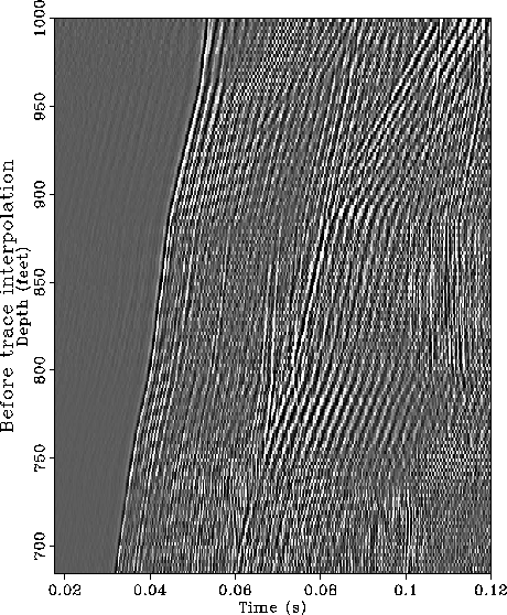
To simulate data with a 2-foot sampling interval in depth, we
decimated the original gather in space. The result is displayed in
Figure ![[*]](http://sepwww.stanford.edu/latex2html/cross_ref_motif.gif) . The steepest linear events representing
tube waves that travel up and down in the receiver well become aliased in space.
Because the tube waves interfere with useful events they should be
removed by dip filtering during the preprocessing.
However, existing dip-filtering techniques do not work for
such spatially aliased data. Therefore, we need to do
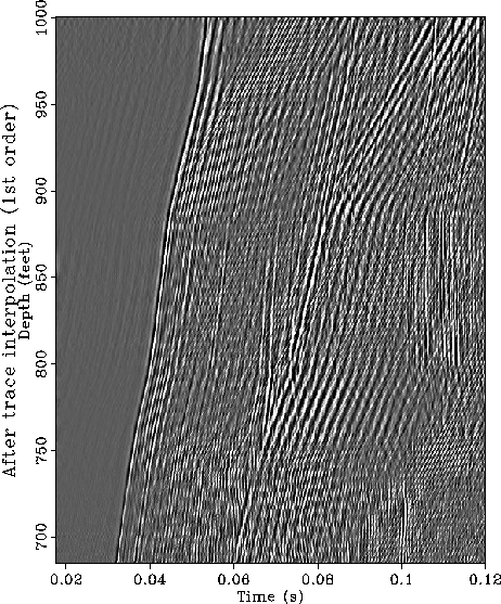
interpolation before dip filtering. Figure
displays the result of the first-order trace interpolation.
We used overlapping subwindows of 128 samples in time and 32 samples
in space. The prediction filter length is 6.
A close look at two locations where strong tube-waves
present--at arrival time 0.07 second and depth 970 feet, and at arrival time
1.1 second and depth 740 feet--shows that seriously aliased tube waves
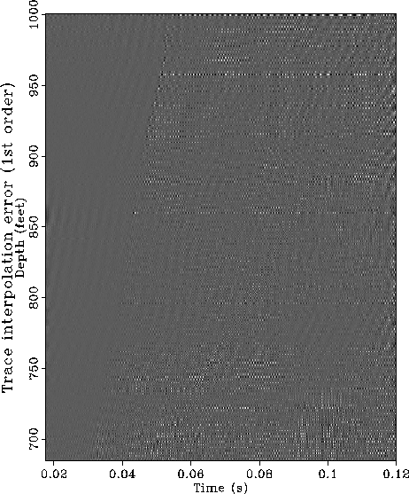
are correctly interpolated. To check the overall quality of interpolation,
we subtract the interpolated gather from the original gather.
Figure shows that the interpolation errors
are generally small and, more importantly, that the distribution of errors
is quite random, that is, the spatial coherence of the interpolation errors
is weak. Large errors appear only along the boundaries of the gather, with
the exception of the trace recorded at the depth of 960 feet. After checking
the original data, we found that this trace was misshifted in the original
gather. Thus we consider the result satisfactory.
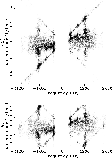
Figure displays the 2-D spectra of the gather before and after
interpolation. Figure compares the results of removing
tube waves before and after interpolation. The depth sampling intervals are
3 feet before interpolation and 1 foot after interpolation.
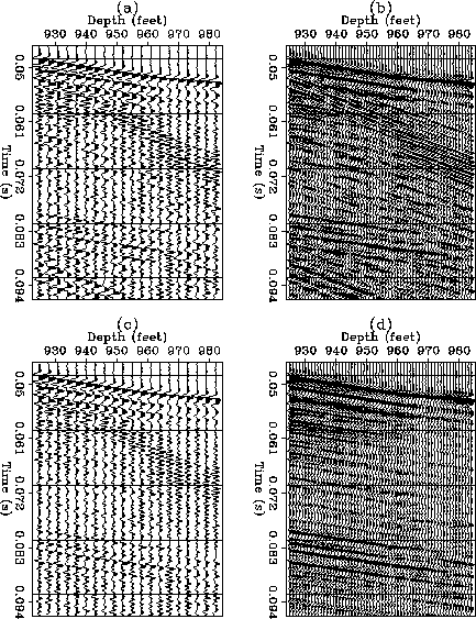
Dip filtering is actually
performed in the slant-stack domain. Before interpolation, the steep
events cannot be filtered out because the dips of the aliased event are
ambiguous. After interpolation, the dips of all events are well defined.
Consequently, tube waves are effectively removed. Many events that
are originally blocked by tube waves are now visible.
cwlsub1
. The steepest linear events representing
tube waves that travel up and down in the receiver well become aliased in space.
Because the tube waves interfere with useful events they should be
removed by dip filtering during the preprocessing.
However, existing dip-filtering techniques do not work for
such spatially aliased data. Therefore, we need to do
interpolation before dip filtering. Figure
displays the result of the first-order trace interpolation.
We used overlapping subwindows of 128 samples in time and 32 samples
in space. The prediction filter length is 6.
A close look at two locations where strong tube-waves
present--at arrival time 0.07 second and depth 970 feet, and at arrival time
1.1 second and depth 740 feet--shows that seriously aliased tube waves
are correctly interpolated. To check the overall quality of interpolation,
we subtract the interpolated gather from the original gather.
Figure shows that the interpolation errors
are generally small and, more importantly, that the distribution of errors
is quite random, that is, the spatial coherence of the interpolation errors
is weak. Large errors appear only along the boundaries of the gather, with
the exception of the trace recorded at the depth of 960 feet. After checking
the original data, we found that this trace was misshifted in the original
gather. Thus we consider the result satisfactory.
Figure displays the 2-D spectra of the gather before and after
interpolation. Figure compares the results of removing
tube waves before and after interpolation. The depth sampling intervals are
3 feet before interpolation and 1 foot after interpolation.
Dip filtering is actually
performed in the slant-stack domain. Before interpolation, the steep
events cannot be filtered out because the dips of the aliased event are
ambiguous. After interpolation, the dips of all events are well defined.
Consequently, tube waves are effectively removed. Many events that
are originally blocked by tube waves are now visible.
cwlsub1
Figure 6 A decimated shot gather that was recorded in a cross-well experiment.
The spatial sampling interval is 2 feet. The shot depth is 540 feet.


 cwlint1
Figure 7 The shot gather after the first-order interpolation. The spatial
sampling interval becomes 1 foot.
cwlerr1
Figure 8 Interpolation errors.
cwlintspc1
Figure 9 Comparison of 2-D spectra: (a) before interpolation,
(b) after interpolation with Spitz's algorithm.
cwlcom
Figure 10 Results of removing tube waves: (a) data before interpolation,
(b) data after interpolation, (c) output of dip filtering before interpolation,
(d) output of dip filtering after interpolation.
Next: CONCLUSIONS
Up: NUMERICAL EXAMPLES
Previous: Synthetic data
Stanford Exploration Project
11/18/1997