CHIRP EXAMPLE

A function generally useful with seismic vibrator sources is the ``gated-chirp function''. Within a specified time gate this function is a sinusoid with a time-variable frequency. Here we will take this signal to be defined by

$$f(\tau ) \quad = \quad \left\{ \begin{array} {ll} \sin( 0... ...\tau_{\max} \\ 0 & \quad \mbox{otherwise} \end{array} \right.$$ (1)

The phase $\phi$ and instantaneous frequency $\omega$of this chirp signal is

$$\begin{eqnarray} \phi &=& 0.5\ \omega_{\max} \ \tau^2 / \tau_{\max} \\ \omega &=... ...\phi \over d\tau} \quad = \quad \omega_{\max} \ \tau / \tau_{\max}\end{eqnarray}$$ (2) (3)

which shows that as $\tau$ ranges from to $\tau_{\max}$,the frequency $\omega$ ranges from to $\omega_{\max}$.

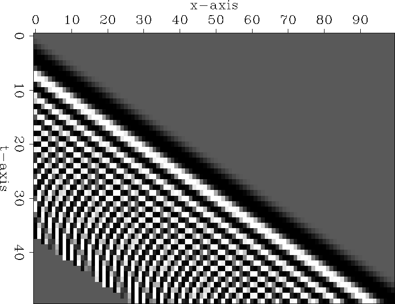
Now consider the chirp signal seen on a wave, say f(t-px). For constant x we see a chirp signal, possibly shifted on the time axis. For constant t we see a chirp function along the x axis, but the -p causes the chirp to be reversed and stretched. Figure 1 shows the chirp wave function f(t-px) for p=0.45 and for $\omega_{\max}=2\pi$.

 

alias2d
Figure 1 A coarsely sampled chirp function on a wavefront.

Since $\omega_{\max}=2\pi$ is double the Nyquist frequency, you see aliasing on the time axis in Figure 1. In other words, along the left edge, the frequency first increases with time until it reaches the Nyquist frequency and then, as frequency goes beyond Nyquist, the apparant frequency decreases. Something else happens on the space axis which is best seen along the bottom edge of the plot. There the frequency sweeps steadily from zero to Nyquist.

Thus, we see that the continuum is different from the sampled world. In a continuum, the function f(t-px) at constant t looks like the same function at constant x except for shifting, reversal, and stretching. In the sampled world we see different functions on each axis. The sampled world matches the continuum only at low frequencies.

In real life, figures like Figure 1 do not arise because it is easy to sample densely enough in time, or to high-cut filter the data before sampling it. Figure 1 might be a starting point, however, for studying whether and why travel times of waves can be mapped more precisely than the time sampling interval, $\Delta t$.

To convert Figure 1 to something closer to real life we need only change the given figure from |p|<1 to |p|>1. There is no need for another figure though because we need only interchange the time axis and the space axis in Figure 1. This leads to the most elementary description of spatial aliasing: Spatial aliasing is when a spatial frequency looks lower than it would if the data were more densely sampled in space. What we seek now are more analytic handles on spatial aliasing.