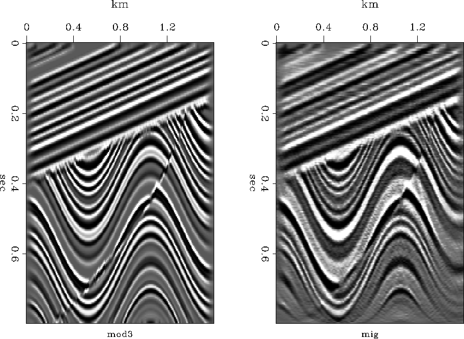
![[*]](http://sepwww.stanford.edu/latex2html/cross_ref_motif.gif) yields the result in Figure 2.
yields the result in Figure 2.
Reconstructing the earth model with the conjugate option in kirchfast() ![[*]](http://sepwww.stanford.edu/latex2html/cross_ref_motif.gif) yields the result in Figure 2.
yields the result in Figure 2.
 |
Difficult migrations are well known for producing semicircular reflectors. Here we have controlled everything fairly well so none are obvious, but on a video screen I see some semicircles.
Next is the problem of the spectrum.
Notice in Figure 2 that the reconstruction
lacks the sharp crispness of the original.
It can be shown mathematically
that the spectrum of our reconstruction
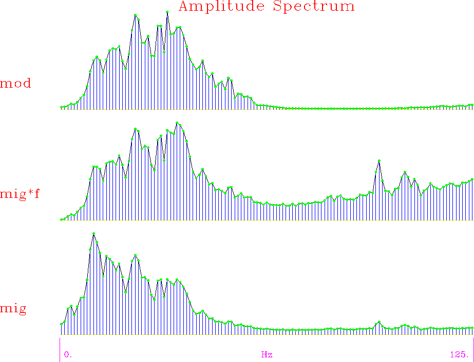
loses high frequencies by a scale of about ![]() .Philosophically, we can think of the integration as boosting
low frequencies.
Figure 3 shows the average over x
of the relevant spectra.
.Philosophically, we can think of the integration as boosting
low frequencies.
Figure 3 shows the average over x
of the relevant spectra.
|
kirspec
Figure 3 Top is the spectrum of the left side of Figure 2. Bottom is the spectrum of the right side of Figure 2. Middle is bottom times frequency. |  |
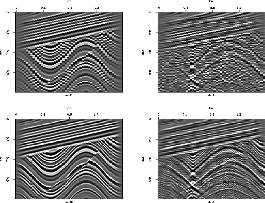
Neither of these Kirchhoff codes addresses the issue of spatial aliasing. Spatial aliasing is a vexing issue of numerical analysis. The Kirchhoff codes shown here do not work as expected unless the space mesh size is suitably more refined than the time mesh. Figure 4 shows an example of forward modeling with a spatial mesh of 50 and 100 points.
 |
![[*]](http://sepwww.stanford.edu/latex2html/cross_ref_motif.gif) does interpolation by moving values
to the nearest neighbor of the theoretical location.
Had we taken the trouble to interpolate the two nearest points,
our results would have been a little better,
but the basic problem (resolved in jon/res/trimo) would remain.
does interpolation by moving values
to the nearest neighbor of the theoretical location.
Had we taken the trouble to interpolate the two nearest points,
our results would have been a little better,
but the basic problem (resolved in jon/res/trimo) would remain.