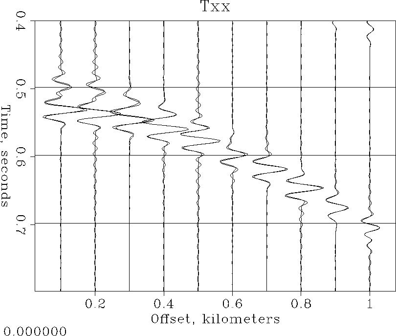
![[*]](http://sepwww.stanford.edu/latex2html/cross_ref_motif.gif) shows what happens
if you subsample by a factor of four and reinterpolate back using
our Fourier-domain method. (This time we subsampled too far and our
sinc functions got out of control!)
shows what happens
if you subsample by a factor of four and reinterpolate back using
our Fourier-domain method. (This time we subsampled too far and our
sinc functions got out of control!)
We hope that you are already getting somewhat familiar with SEPlib, so from now on we will not explain all the programs in depth as we did before. Most of the programs are self-explanatory in these examples, and you should not forget about their self documentation (just type the name of the program). So let's start, and good luck!
Start by subsampling the data using Window:
Window < Txx.H j1=2 > Txx_sub.HThis decimates the
1 (time) axis by a factor of 2.
Now suppose we accidentally lost the original data and only had the subsampled version left. If the original data was sufficiently oversampled, we should be able to recover the original by transforming to the Fourier domain, padding, and transforming back. Can we perform this sequence using only available SEPlib utilities?
The Fourier transform utility, ``Ft3d'', demands complex input
(it will barf with ``Ft3d: esize must be 8'' if it doesn't get it),
so we first convert from Real to Complex using Rtoc. Then
we can use Ft3d to do the Fourier transform, with a
command-line parameter to tell it we only want to transform
over the 1 axis:
Rtoc < Txx_sub.H | Ft3d sign1=1 > Txx_Fft.HYou may enjoy examing a plot of Complex absolute value in the frequency domain:
Cabs < Txx_Fft.H | Wiggle | Tube
Now we pad from 512 back to 1024 points, inverse Fourier-transform, take the real part, make a Wiggle plot, and plot it (whew)!
Pad < Txx_Fft.H n1=1024 | Ft3d | Real | Wiggle par=plotpar | Tube(We didn't have to tell
Ft3d what to do because it looks at
the parameters from its last run preserved in the history file, and
by default does the inverse.)
And the resulting plot is... JUNK!
Well, of course. ``Pad'' is a stupid program that just appends
enough zeroes onto the end of a given axis to make a dataset of the
requested size. That's fine for some applications, but not for
this one.
To do the job right we have to separate out the positive
frequencies, negative frequencies, DC, and Nyquist and make sure they all
end up in the right places. Zero frequency is in slot 0.
We have 512 frequency points, so the positive
frequencies must be in slots 1 to 255, the Nyquist is in slot 256, and
the negative frequencies are in slots 257 to 511.
(Almost all SEPlib programs
use C numbering notation, not FORTRAN numbering notation...
arrays start with element 0, not 1.)
Let's separate them all out.
Window < Txx_Fft.H n1=1 f1=0 squeeze=n > DC.H
Window < Txx_Fft.H n1=255 f1=1 squeeze=n > Pos.H
Window < Txx_Fft.H n1=1 f1=256 squeeze=n > Nyquist.H
Window < Txx_Fft.H n1=255 f1=257 squeeze=n > Neg.H
(If the
1 axis on output would have length 1,
Window by default helpfully swaps it around
and makes it the 2 axis. For this case it is not helpful.
The ``squeeze=n'' option prevents this.)
The Nyquist has to go in twice, so we need to divide it by two:
Add Nyquist.H scale=.5 > Nyquisto2.HAnd finally we put it back together with the padding in the middle, and bring it back to the time domain:
Merge axis=1 space=n DC.H Pos.H Nyquisto2.H | Pad > Junk n1=768
Merge axis=1 space=n Junk Nyquisto2.H Neg.H > Txx_Fft2.H
Ft3d < Txx_Fft2.H | Real > Junk
Add Junk scale=1.414213562 > Txx_resamp.H
Rm Junk DC.H Pos.H Nyquisto2.H Neg.H Txx_Fft.H
(
Merge by default helpfully inserts a zero trace between
merged blocks, so you can see where the boundaries are.
``space=n'' turns this off. We have to rescale by Compare the original and reconstructed data by doing
Cat Txx.H Txx_resamp.H | Wiggle par=plotpar | TubeAs you (hopefully) can see, we appear to have recovered the original dataset exactly.
Hopefully you enjoyed this example and you are ready to try more.
If you are familiar with UNIX you can build a shell script to do all this
automatically so that you don't have to retype it again and again.
If you are really ambitious, create a shell script that lets you specify
the power of two to subsample by. Figure ![[*]](http://sepwww.stanford.edu/latex2html/cross_ref_motif.gif) shows what happens
if you subsample by a factor of four and reinterpolate back using
our Fourier-domain method. (This time we subsampled too far and our
sinc functions got out of control!)
shows what happens
if you subsample by a factor of four and reinterpolate back using
our Fourier-domain method. (This time we subsampled too far and our
sinc functions got out of control!)
 |
Different people use SEPlib programs different ways. Some prefer to type everything themselves as we have been doing here. Some write everything as shell scripts. Others like to do everything from within Makefiles (or Cakefiles). How you use SEPlib is up to you.