THE ALGORITHM

I implement the algorithm in several straightforward one-dimensional modules. The data are partitioned by low-pass filtering and the low-frequency portion is interpolated. The high-frequency (HF) portion of the data is then reconstructed for the interpolated traces. The data are partitioned into small windows in which the interpolation is performed. The windows are then pieced back together to create the final interpolated section. The task of partitioning and re-assembling the data is performed by Claerbout's subroutine patch() Claerbout (1992b).

The whole interpolation scheme can be divided into five discrete modules:

• Each trace is low-pass filtered. By filtering the data in time, the spatially aliased portion of the spectrum is removed.
• The low-pass filtered data are interpolated in space by performing a one-dimensional Fourier transform, zero padding, and performing the inverse transform.
• The low-frequency (LF) data are then cubed in the time domain in order to broaden the spectrum. This is done to both the original and interpolated LF data.
• The cubed LF traces ([f_low(t)]³) are then used to find a shaping filter. For each original trace, a filter b(t) is found such that

  b(t)*[f_low(t)]³=f_all(t)

  where f_all(t) is the wide-band data including high- and low- frequency. This is done using conjugate gradients with the subroutine shp() (Appendix).
• Once the shaping filter is found, it is used to reconstruct the HF data on the interpolated traces.

The cubing operation is used simply to enrichen the spectral content of the interpolated low-frequency data so that the shaping filter can be applied. It was chosen since it is a low order polynomial power which preserves polarity. In a more general formulation the fifth, seventh, etc. powers could be used. Even powers could also be used by forming something like 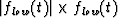$\vert f_{low}(t)\vert\times f_{low}(t)$ so that polarity is preserved.