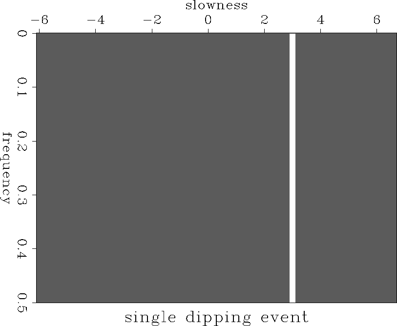
The amplitude spectra displaying in the previous spectrum were created using a ``direct'' slant stack. The transformation to the slant stack domain was performed using the traditional ``sum along lines'' operator plus a rho filter.
![]()
The problems with using this approach have been well documented
Kostov (1990). The limited aperture and sampling in the
x-t domain cause artifacts. Irregular sampling in x is not well
handled by the direct stacking procedure. The alternative is to
perform a least squares inverse slant stack. This method assumes that
we can exactly perform the mapping from ![]() to x-t and casts
the mapping from x-t to
to x-t and casts
the mapping from x-t to ![]() as an inverse problem. This is most
conveniently calculated in the frequency domain.
as an inverse problem. This is most
conveniently calculated in the frequency domain.
The operator that maps from ![]() to
to ![]() is L,
is L,
![]()
![]()
![]()
![]()
![]()
The operator (LHL) has a Toeplitz form when the data is regularly sampled in p. This makes the inversion cheap to solve using Levinson recursion. A problem with this method is that the operator LHL becomes singular when the data is aliased. Kostov suggests two ways to overcome this problem, ``Aliasing can be overcome by using prior information, either in the form of an interval of wavenumbers smaller than twice the Nyquist wavenumber, or by introducing ``a priori'' information via a model-covariance matrix.'' (I would suggest that the first statement can be modified to allow multiple wavenumber intervals as long as the total width does not exceed twice the Nyquist wavenumber and no two intervals occur at positions that are the alias of one another.)
My first solution to the problem is to constrain the solution to be non-zero only in those places that I have defined as unaliased. I define a masking operator, M, that is one where the data is not aliased and zero where it is aliased. I then solve the least squares problem,
![]()
![]()
![]()
![[*]](http://sepwww.stanford.edu/latex2html/cross_ref_motif.gif) shows the
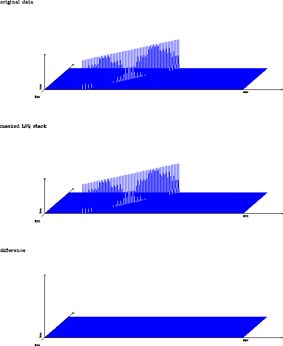
shows the ![[*]](http://sepwww.stanford.edu/latex2html/cross_ref_motif.gif) has three frames. The top frame is the
original x-t domain data. The middle frame is the reconstruction of
the x-t data from the masked least squares inverse slant stack. The
bottom frame is the difference between the two panels plotted at the
same scale. The reconstruction has been completely successful. I am
not limited to reconstructing the data at the original trace spacing,
the data can be modeled in the x-t domain at an arbitrary regular or
irregular trace spacing.
has three frames. The top frame is the
original x-t domain data. The middle frame is the reconstruction of
the x-t data from the masked least squares inverse slant stack. The
bottom frame is the difference between the two panels plotted at the
same scale. The reconstruction has been completely successful. I am
not limited to reconstructing the data at the original trace spacing,
the data can be modeled in the x-t domain at an arbitrary regular or
irregular trace spacing.
|
single-lsq
Figure 5 |  |
 |