SVD (Dongarra, et al., 1979)
was performed on the matrix ![]() after parametrizing the model as described by
equations (3) , (4) and (5).
Pratt and Chapman (1990) suggest a clear way of representing
the resultant singular values and singular vectors in model space
(
after parametrizing the model as described by
equations (3) , (4) and (5).
Pratt and Chapman (1990) suggest a clear way of representing
the resultant singular values and singular vectors in model space
(![]() )
of the matrices involved in tomographic
problems. I will represent my results in a similar fashion including
also in the representation the corresponding singular vectors in data
space (
)
of the matrices involved in tomographic
problems. I will represent my results in a similar fashion including
also in the representation the corresponding singular vectors in data
space (![]() ).
This will help to understand how the data and the model
are resolved by using iterative techniques such as conjugate gradients.
).
This will help to understand how the data and the model
are resolved by using iterative techniques such as conjugate gradients.
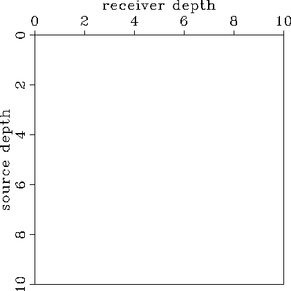
The data space (spanned by the columns of ![]() ) is shown in
Figure
) is shown in
Figure ![[*]](http://sepwww.stanford.edu/latex2html/cross_ref_motif.gif) .
It is a 2-D space of traveltimes where the horizontal axis
contains the receiver depths and the vertical axis contains
the source depths. If the origin of both axes is the same,
the closer a given point is to the main diagonal (near
offset), the
closer is to zero the corresponding ray angle.
.
It is a 2-D space of traveltimes where the horizontal axis
contains the receiver depths and the vertical axis contains
the source depths. If the origin of both axes is the same,
the closer a given point is to the main diagonal (near
offset), the
closer is to zero the corresponding ray angle.
 |
The geometry used to do the SVD for the different
parametrizations is shown in Figure ![[*]](http://sepwww.stanford.edu/latex2html/cross_ref_motif.gif) (Pratt and Chapman, 1990): five sources and five receivers in a constant
slowness medium.
When the model is isotropic, the matrix
(Pratt and Chapman, 1990): five sources and five receivers in a constant
slowness medium.
When the model is isotropic, the matrix ![]() only depends
on the ray geometry and when the model is anisotropic,
only depends
on the ray geometry and when the model is anisotropic,
![]() depends on both the ray geometry and
the slowness model (constant in this case).
depends on both the ray geometry and
the slowness model (constant in this case).
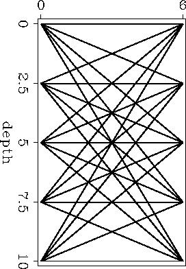 |
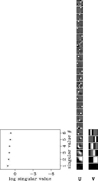
Figure ![[*]](http://sepwww.stanford.edu/latex2html/cross_ref_motif.gif) shows the SVD when the model is
discretized using 6 horizontal isotropic layers (equation 3).
Notice that the
differences among the singular values are small.
The largest singular values correspond to singular vectors in
data and model space whose components are roughly
of the same magnitude.
We observe that with this
parametrization only some ``big structures'' (averages)
in data space can be explained whereas in
model space all the parameters can be resolved well.
By representing the data space as described by Figure 1,
it is possible to identify
which traveltimes belong
to the null space and therefore, cannot be resolved. Errors in these
particular
traveltimes (noise) will also have little or no effect in the solution.
shows the SVD when the model is
discretized using 6 horizontal isotropic layers (equation 3).
Notice that the
differences among the singular values are small.
The largest singular values correspond to singular vectors in
data and model space whose components are roughly
of the same magnitude.
We observe that with this
parametrization only some ``big structures'' (averages)
in data space can be explained whereas in
model space all the parameters can be resolved well.
By representing the data space as described by Figure 1,
it is possible to identify
which traveltimes belong
to the null space and therefore, cannot be resolved. Errors in these
particular
traveltimes (noise) will also have little or no effect in the solution.
 |
When lateral variations are allowed in the previous
parameterization results a matrix ![]() whose
SVD
is shown in Figure
whose
SVD
is shown in Figure ![[*]](http://sepwww.stanford.edu/latex2html/cross_ref_motif.gif) . The largest singular value
corresponds roughly to horizontal layers (in model space)
and non-horizontal rays (in data space). As the singular
values
decrease, the eigenvectors in model space tend
to contain more horizontal variations and the eigenvectors
in data space tend to expand near and far
offsets alternatively (diagonal and non-diagonal structures).
The null space of the
problem corresponds to ``pure''
horizontal variations in model space and
high frequency variations
data space (rapid changes among nearby traveltimes).
These vectors in the null space of the data are probably
not a problem in real applications because if the real velocities do not change
rapidly, high frequency variations are
unlikely to be found in the measured traveltimes.
The presence of noise introduces high frequency variations in the data.
Unfortunately,
these type of variations are
not confined to the null space of the data but are present
in singular vectors corresponding to
larger singular values. Therefore, in some
applications it might be necessary to damp the effect of singular
values larger than those contained in the null space in order to attenuate
the effect of certain components of the noise.
. The largest singular value
corresponds roughly to horizontal layers (in model space)
and non-horizontal rays (in data space). As the singular
values
decrease, the eigenvectors in model space tend
to contain more horizontal variations and the eigenvectors
in data space tend to expand near and far
offsets alternatively (diagonal and non-diagonal structures).
The null space of the
problem corresponds to ``pure''
horizontal variations in model space and
high frequency variations
data space (rapid changes among nearby traveltimes).
These vectors in the null space of the data are probably
not a problem in real applications because if the real velocities do not change
rapidly, high frequency variations are
unlikely to be found in the measured traveltimes.
The presence of noise introduces high frequency variations in the data.
Unfortunately,
these type of variations are
not confined to the null space of the data but are present
in singular vectors corresponding to
larger singular values. Therefore, in some
applications it might be necessary to damp the effect of singular
values larger than those contained in the null space in order to attenuate
the effect of certain components of the noise.
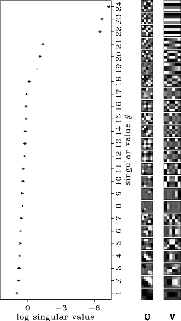 |
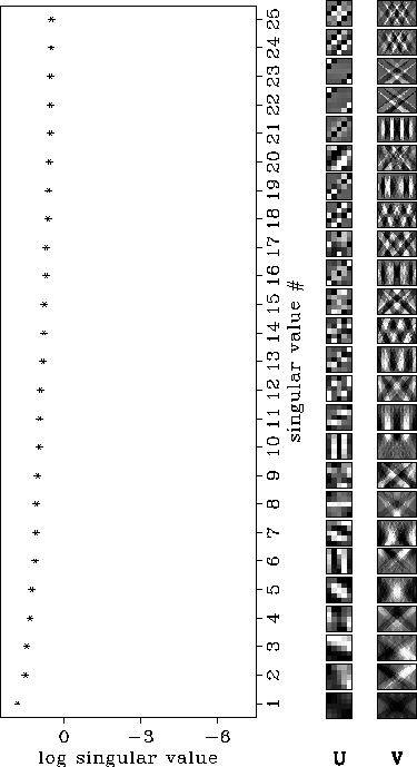
Figure ![[*]](http://sepwww.stanford.edu/latex2html/cross_ref_motif.gif) shows the SVD of the matrix that result after
discretizing the model and computing the data using natural pixels (equation
4).
We notice immediately that the matrix for the natural pixels is much better
conditioned than the one obtained with square pixels
(Figure
shows the SVD of the matrix that result after
discretizing the model and computing the data using natural pixels (equation
4).
We notice immediately that the matrix for the natural pixels is much better
conditioned than the one obtained with square pixels
(Figure ![[*]](http://sepwww.stanford.edu/latex2html/cross_ref_motif.gif) ). The singular vectors in data space that
correspond to the largest singular value are almost identical
for both discretizations. However, the ways those data are distributed
in the model are different for the different discretizations.
For all the eigenvectors in Figure
). The singular vectors in data space that
correspond to the largest singular value are almost identical
for both discretizations. However, the ways those data are distributed
in the model are different for the different discretizations.
For all the eigenvectors in Figure ![[*]](http://sepwww.stanford.edu/latex2html/cross_ref_motif.gif) there is a clear correspondency between the structures represented in data
and model space, unlike the eigenvectors in Figure
there is a clear correspondency between the structures represented in data
and model space, unlike the eigenvectors in Figure ![[*]](http://sepwww.stanford.edu/latex2html/cross_ref_motif.gif) .
With the natural pixels all the parameters and data
can be resolved because
the discretization does not introduce another null space in the problem
(different to the null space of the measurements), whereas the discretization
of the model
in square pixels does.
.
With the natural pixels all the parameters and data
can be resolved because
the discretization does not introduce another null space in the problem
(different to the null space of the measurements), whereas the discretization
of the model
in square pixels does.
 |
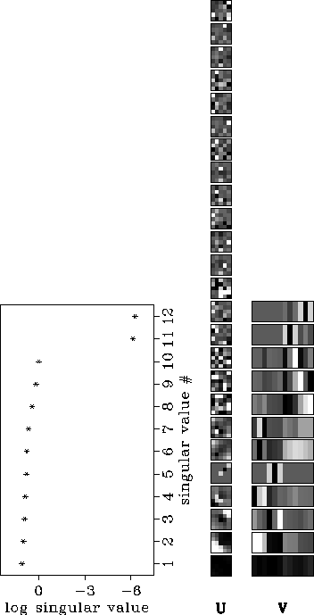
The SVD for a 1-D anisotropic parametrization (equation 5) is shown
in Figure ![[*]](http://sepwww.stanford.edu/latex2html/cross_ref_motif.gif) .
The
upper half of each eigenvector in model space
corresponds to Sx and the lower half corresponds to Sz.
We observe that the largest singular values correspond to
Sx in model space
and in data space the behavior is similar to the
isotropic 1-D case. The null space of the model is spanned
by vectors that only contain information about Sz.
.
The
upper half of each eigenvector in model space
corresponds to Sx and the lower half corresponds to Sz.
We observe that the largest singular values correspond to
Sx in model space
and in data space the behavior is similar to the
isotropic 1-D case. The null space of the model is spanned
by vectors that only contain information about Sz.
 |
 |
 |
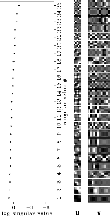
Figure ![[*]](http://sepwww.stanford.edu/latex2html/cross_ref_motif.gif) shows the SVD
when the model is 2-D anisotropic. The result is nearly
a combination of the previous ones in model space,
namely, vertical variations in Sx correspond to the
largest singular values and horizontal variations in Sz
to the smallest ones. The null space of the model (Figure
shows the SVD
when the model is 2-D anisotropic. The result is nearly
a combination of the previous ones in model space,
namely, vertical variations in Sx correspond to the
largest singular values and horizontal variations in Sz
to the smallest ones. The null space of the model (Figure ![[*]](http://sepwww.stanford.edu/latex2html/cross_ref_motif.gif) )
is formed
almost entirely by ``unit'' vectors that describe Sz.
For this reason,
in the synthetic and real data
applications shown in Michelena and Muir (1991), the resolution
of the vertical component of the slowness is poor when compared with
the resolution
of the horizontal component. As expected, Sz is poorly defined by the
cross-well recording
geometry.
Note that by increasing the number of model parameters the condition number
of the matrix diminishes when compared with the one of
the matrix for the isotropic case
(Figure 4).
)
is formed
almost entirely by ``unit'' vectors that describe Sz.
For this reason,
in the synthetic and real data
applications shown in Michelena and Muir (1991), the resolution
of the vertical component of the slowness is poor when compared with
the resolution
of the horizontal component. As expected, Sz is poorly defined by the
cross-well recording
geometry.
Note that by increasing the number of model parameters the condition number
of the matrix diminishes when compared with the one of
the matrix for the isotropic case
(Figure 4).