Traveltimes and rays

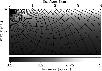
The traveltime calculation algorithm can handle virtually arbitrary slowness models. Figure shows the results for a medium in which velocity linearly increases with depth. The velocity gradient is 1.5 1/sec. The background of this figure shows the slowness model. I plot contour lines of the traveltimes on this background. The contour lines of the traveltimes are the trajectories of the wavefronts. We see that the wavefronts are stretched downward because the slowness decreases with depth. Because the function $\gamma(x,z)$ defined in equation (14) is constant along each ray, I plot the contour lines of this function to show the rays. The values of the contours are uniformly spaced so that the rays plotted are shot with uniform take-off angles. As expected, we see many overturned rays.

 

ttmraygra
Figure 2 Wavefronts and rays for a model with a velocity function that is linearly increasing as a function of depth. The background shows the slowness model. The source is at the upper left corner of the figure. The traveltime contour lines are drawn at 0.1 second intervals.

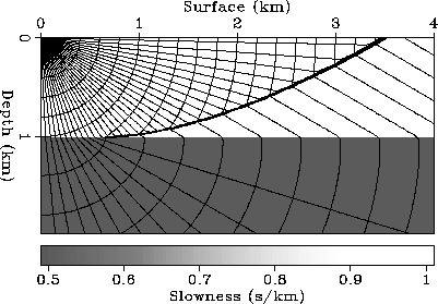
The slowness model in the second example is a medium with two layers. The velocity contrast between the top layer and the bottom layer is 1 to 2. Figure shows the results of the calculations. The content of this figure is similar to Figure . We see the first arrivals associated with both transmitted waves and refracted waves. We see the transmitted rays but not the rays refracted along the interface. This is because all the refracted rays originate from a single ray; therefore the values of the function $\gamma(x,z)$ along all the refracted rays are equal. The thick curve that appears in the top layer is the boundary that separates the first arrivals from the transmitted waves and the refracted waves.

 

ttmraylay
Figure 3 Wavefronts and rays for a model with two constant-velocity layers. The background shows the slowness model. The source is at the upper left corner of the figure. The traveltime contour lines are drawn at 0.2 second intervals.

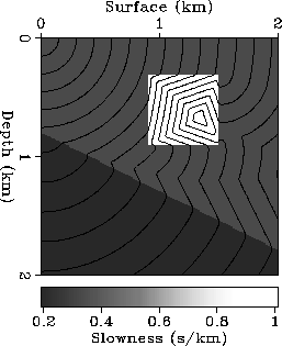
The final example for the traveltime calculation uses a slowness model containing an anomaly with large velocity contrast. The results of the calculations are shown in Figure . The looping contour lines within the anomaly are due to the finite grid sizes. Clearly, in the lower right part of the anomaly, the first arrivals propagate back toward the source. This part is calculated by backward extrapolation.

 

ttmrayrec
Figure 4 Wavefronts for a model with a sharply-contrasted anomaly. The background shows the slowness model. The source is at the upper left corner of the figure. The traveltime contour lines are drawn at 0.05 second intervals.