Next: EXAMPLES
Up: IMPLEMENTATION
Previous: The free boundary and
The spatial operator was designed to be grid-centered of eighth
order (9 points).
It can be decomposed in three parts for each component:
|  |
(10) |
where
| 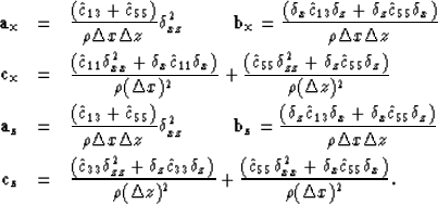 |
|
| |
| |
| (11) |
 and
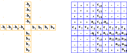
and  are antisymmetric but
  has no particular
symmetry (except in homogeneous media); and their form is represented
in Figure
has no particular
symmetry (except in homogeneous media); and their form is represented
in Figure ![[*]](http://sepwww.stanford.edu/latex2html/cross_ref_motif.gif) . The
. The  operators are grid-centered, normalized,
bi-dimensional difference stars.
spaceop
operators are grid-centered, normalized,
bi-dimensional difference stars.
spaceop
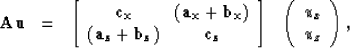
Figure 4 Spatial difference operators described by equation (11).

The temporal updating uses the operator  described
in Cunha (1991) in this report. To obtain the wavefield and its
time derivative at time time
described
in Cunha (1991) in this report. To obtain the wavefield and its
time derivative at time time  only requires information
from time t, that is,
only requires information
from time t, that is,
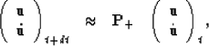
where the forward time-propagation operator  has the form
| ![\begin{displaymath}
{\bf P_{+}} = \left[ \begin{array}
{ccc} {\bf I} + {{\bf A} ...
... \over 2} dt^2 + {{\bf A}^2 \over 24} dt^4 \end{array} \right],\end{displaymath}](img26.gif) |
(12) |
which represents a fourth order approximation in time.
Next: EXAMPLES
Up: IMPLEMENTATION
Previous: The free boundary and
Stanford Exploration Project
12/18/1997