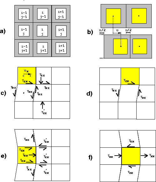
It is sufficient to analyze the dynamics associated with the four
basic displacements represented in Figures ![[*]](http://sepwww.stanford.edu/latex2html/cross_ref_motif.gif) -c to
-c to ![[*]](http://sepwww.stanford.edu/latex2html/cross_ref_motif.gif) -f
since all the other cases can be easily derived from them.
The following items refer to each of those figures in turn.
-f
since all the other cases can be easily derived from them.
The following items refer to each of those figures in turn.
- case c
A displacement ux in cell [i-1,j-1] originates a shear traction Tzx
between [i-1,j-1] and [i-1,j] (the traction applied by the first on
the second is represented in the figure).

where Lx is the x dimension of an undeformed cell.
The rotational equilibrium requires that the total momentum
applied to [i-1,j] be zero. Therefore

The same equilibrium condition in [i,j], requires that the same
shear traction Txz be applied on it by [i,j-1].
The compression of [i,j-1] by ux/2 creates a compressional
traction Tzz (associated with Young's moduli) between [i,j-1] and
[i,j), while the asymmetrical compression of [i,j] produces
a compressional traction  between [i,j] and
[i,j+1] given by the equations

The total force applied in [i,j] due to [i-1,j-1]'s displacement
then has the following components:

- case d
A displacement ux in cell [i,j-1] creates a shear traction Tzx
between [i,j-1] and [i,j], whose magnitude is given by the equation

This traction will be responsible for the only net force applied in [i,j],
because the two shear tractions between [i,j] and [i-1,j], and between
[i,j] and [i+1,j] compensate each other as well as the two compressional
tractions (not represented in the figure) acting in the same interfaces.
The total force applied in [i,j] due to [i,j-1]'s displacement
has only an x component, as follows:

- case e
A displacement ux in cell [i-1,j] creates a compressional
traction Txx between [i-1,j] and [i,j], and a shear traction
Tzx between [i-1,j] and [i-1,j-1] whose magnitudes are given by
the equations

Applying the equilibrium conditions in [i-1,j-1] and [i,j-1], it
follows that  .This traction is responsible for the only net force applied in
[i,j], because the two shear tractions between [i,j] and [i-1,j], and
[i,j] and [i+1,j] compensate each other as well as the two compressional
tractions (not represented in the figure) acting in the same interfaces.
The total force applied in [i,j] caused by [i-1,j]'s displacement
also has only an x component:

- case f
A displacement ux in cell [i,j] creates compressional
tractions Txx between [i-1,j] and [i,j], and between [i,j] and
[i+1,j], and a shear traction Tzx between [i,j-1] and [i,j+1],
whose magnitudes are given by the following equations:

The total force applied in [i,j] caused by [i,j]'s displacement
also has only an x component, as follows:

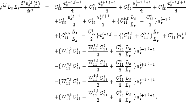
For the more general heterogeneous case, some definitions are required
to simplify the equations of motion:
![[*]](http://sepwww.stanford.edu/latex2html/cross_ref_motif.gif) -a shows the 2-D elastic equivalent of the spring-mass
model described in the paper. The medium is constituted by square cells
with the mass concentrated in the center of the cell, and the elastic,
massless part located at the boundaries. This elastic part is responsible
for all the interaction between adjacent cells. As in the 1-D case, only
adjacent cells can interact with each other. Therefore, the dynamics of
cell [i,j] in Figure
-a shows the 2-D elastic equivalent of the spring-mass
model described in the paper. The medium is constituted by square cells
with the mass concentrated in the center of the cell, and the elastic,
massless part located at the boundaries. This elastic part is responsible
for all the interaction between adjacent cells. As in the 1-D case, only
adjacent cells can interact with each other. Therefore, the dynamics of
cell [i,j] in Figure ![[*]](http://sepwww.stanford.edu/latex2html/cross_ref_motif.gif) -a is controlled only by its own
position, and the positions of its eight neighbor cells.
-a is controlled only by its own
position, and the positions of its eight neighbor cells.


