Next: CONCLUSIONS
Up: USING PREDICTION TO DESIGN
Previous: USING PREDICTION TO DESIGN
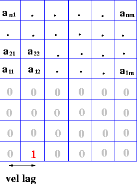
Figure ![[*]](http://sepwww.stanford.edu/latex2html/cross_ref_motif.gif) shows the form of the desired prediction-error
operator in the velocity domain. The prediction lags in the velocity
and time directions and the filter size are controlled by the
particular characteristics of the dataset, following the same basic
designing rules as with the standard 1-D prediction error filter. The
coefficients aij are defined by a power minimization criterion
(Claerbout, 1991). Therefore, if
shows the form of the desired prediction-error
operator in the velocity domain. The prediction lags in the velocity
and time directions and the filter size are controlled by the
particular characteristics of the dataset, following the same basic
designing rules as with the standard 1-D prediction error filter. The
coefficients aij are defined by a power minimization criterion
(Claerbout, 1991). Therefore, if  is the semblance of the
original data and
is the semblance of the
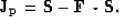
original data and  is the prediction filter, the coefficients
of the filter are obtained by minimizing the L2 error of
equation (6), as follows:
is the prediction filter, the coefficients
of the filter are obtained by minimizing the L2 error of
equation (6), as follows:
|  |
(6) |
predoper
Figure 4 The prediction-error filter for suppressing the regions of the velocity
semblance spectrum that are associated with primary reflections.
|
|  |

realoper
Figure 5 The estimated prediction-error filter for the synthetic data of
Figure -b.
|
|  |


Once the filter coefficients are defined, the weighting operator  is obtained by
|  |
(7) |
Because of the large size of the problem to be solved in
equation (6) and since the semblance is a smooth function
of time, it is convenient to subsample S in time before solving
equation (6) and applying equation (7).
The resulting operator is then interpolated to the original
time sampling interval. The prediction-error filter estimated for
the synthetic data of Figure -b is shown in
Figure .
Figure compares the original semblance with
the result of applying the prediction operator to it
for the synthetic dataset of Figure . It is impressive
that the filter was able to correctly predict the different multiples
patterns present in the data. None of the primaries are visible on
the output. Figure -a shows the window function  constructed from , and Figure -b shows the
semblance spectrum of the synthetic data after 15 iterations
of the optimization process using as the window function.
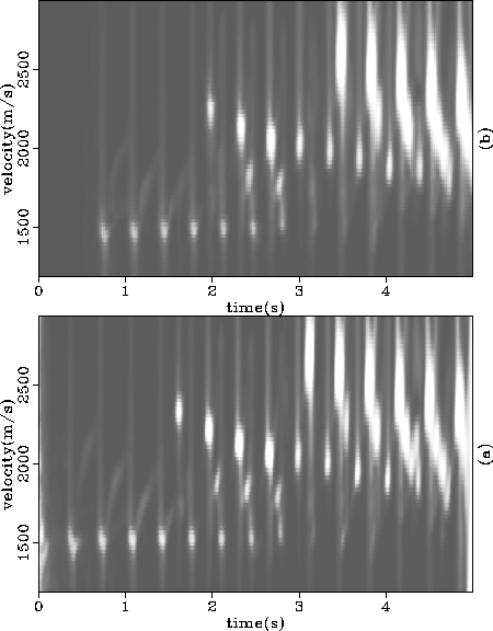
In -b the events associated with reverberations are barely
visible. Most importantly, the parts of the spectrum associated
with the converted waves were preserved, as show the events at 2.05, 2.5,
and 4.3 seconds.
constructed from , and Figure -b shows the
semblance spectrum of the synthetic data after 15 iterations
of the optimization process using as the window function.
In -b the events associated with reverberations are barely
visible. Most importantly, the parts of the spectrum associated
with the converted waves were preserved, as show the events at 2.05, 2.5,
and 4.3 seconds.
sempred
Figure 6 (a) The smoothed semblance spectrum of the data of
Figure and (b) the output of the
prediction operator applied to it.
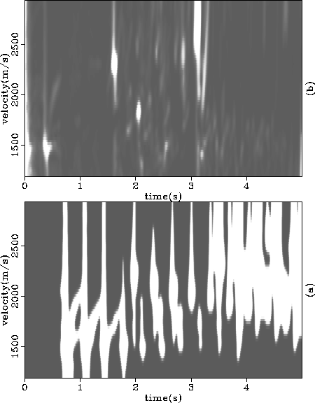
semwind
Figure 7 (a)The window function constructed from the predicted semblance
spectrum shown in Figure -b. (b) The semblance
spectrum of the output of the multiples suppression scheme, using
(a) as the window function.
A comparison of the output of the optimization process with the
``ideal" multiple free data (Figure ) shows that not
only have the multiples been substantially attenuated, but also the
amplitude and phase of the primaries were correctly preserved, including
the weak, low-velocity converted waves.
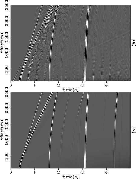
predrm
Figure 8 (a) Synthetic data, free of surface related reverberation (same
as Figure -a). (b) The output of the
multiples suppression scheme applied to the synthetic data of
Figure -b, when the prediction-designed
function of Figure -a is used as the window operator.
Next: CONCLUSIONS
Up: USING PREDICTION TO DESIGN
Previous: USING PREDICTION TO DESIGN
Stanford Exploration Project
12/18/1997