The simplest inversion that we can possibly do is assuming that the medium is homogeneous isotropic. What we obtain is the mean velocity (equation (7)), in this case Viso=8452 ft/sec. The next step is to assume that the model is still homogeneous but elliptically anisotropic. Using equation (8) we find that Vx = 8586 ft/sec and Vz = 8079 ft/sec. Notice that for this particular recording geometry (Figure 9), Viso is closer to Vx than to Vz, which means that the ``averaging'' of the horizontal and vertical directions that the isotropic inversion implicitly does is not a simple arithmetic average. When the model is also heterogeneous, the same conclusion may be drawn as it will be show later.
To measure the goodness of the fit between measured and calculated traveltimes, we use the mean-absolute value of the mismatch
 |
(12) |
When the estimated Viso in the homogeneous model is used to compute synthetic traveltimes, error= 1.04 ms. When the model is homogeneous anisotropic, error= 0.94 ms.
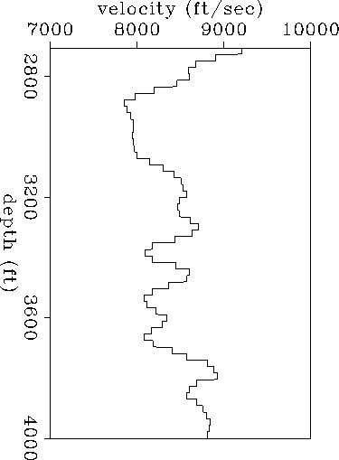
The result of the isotropic inversion assuming a layered medium
is shown in Figure ![[*]](http://sepwww.stanford.edu/latex2html/cross_ref_motif.gif) . Only traveltimes corresponding to rays
below 2705 ft and above 4000 ft were used. This depth interval
was discretized in
60 horizontal layers of equal thickness (21.583 ft). Straight rays
were used to compute synthetic traveltimes since small velocity
variations are expected in this site (Harris et al., 1990b).
Conjugate gradients
iterations (40) were performed until no appreciable changes were
seen neither in the model nor in the mean-absolute value of the
error (equation (12)). This corresponds to reaching
the flat part of the hills in Figure (5). For the model
shown in Figure
. Only traveltimes corresponding to rays
below 2705 ft and above 4000 ft were used. This depth interval
was discretized in
60 horizontal layers of equal thickness (21.583 ft). Straight rays
were used to compute synthetic traveltimes since small velocity
variations are expected in this site (Harris et al., 1990b).
Conjugate gradients
iterations (40) were performed until no appreciable changes were
seen neither in the model nor in the mean-absolute value of the
error (equation (12)). This corresponds to reaching
the flat part of the hills in Figure (5). For the model
shown in Figure ![[*]](http://sepwww.stanford.edu/latex2html/cross_ref_motif.gif) , error = 0.67 ms.
, error = 0.67 ms.
 |
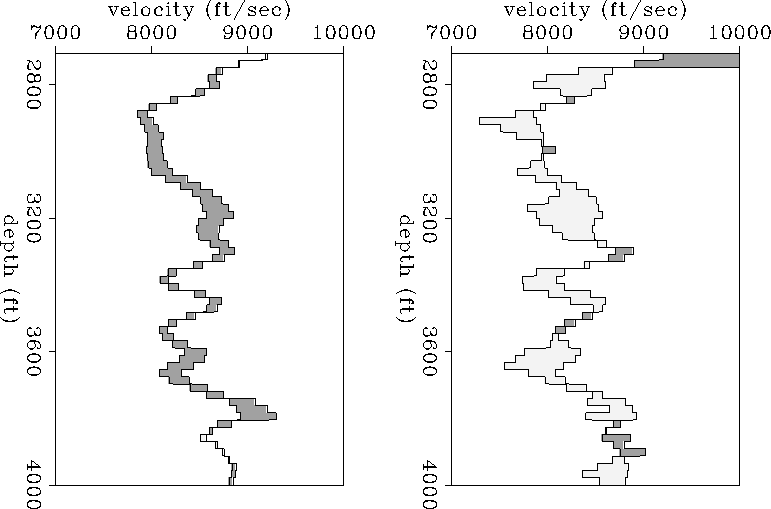
Now, we allow the model to be anisotropic. The result of the inversion
is shown in Figure ![[*]](http://sepwww.stanford.edu/latex2html/cross_ref_motif.gif) . For traveltimes computed
through this model, error=0.59 ms.
The thick curve represents the
horizontal velocity and the thin one represents the vertical velocity. The
first thing we notice is that as expected Vx is generally larger than
Vz. Figure
. For traveltimes computed
through this model, error=0.59 ms.
The thick curve represents the
horizontal velocity and the thin one represents the vertical velocity. The
first thing we notice is that as expected Vx is generally larger than
Vz. Figure ![[*]](http://sepwww.stanford.edu/latex2html/cross_ref_motif.gif) compares Vx and Vz with Viso. In general, Viso
is closer to Vx than it is to Vz, which is consistent with the previous
the results of the inversion assuming an homogeneous medium. This means
that for the type of recording geometry used (ray angles between
and
compares Vx and Vz with Viso. In general, Viso
is closer to Vx than it is to Vz, which is consistent with the previous
the results of the inversion assuming an homogeneous medium. This means
that for the type of recording geometry used (ray angles between
and ![]() degrees) the isotropic inversion is affected primarily
by the horizontal component of the velocity. Since there are fewer rays
at large angles, the isotropic inversion is less constrained by them. However,
rays at large angles contain independent information that might be
important to improve horizontal resolution in 2-D models.
degrees) the isotropic inversion is affected primarily
by the horizontal component of the velocity. Since there are fewer rays
at large angles, the isotropic inversion is less constrained by them. However,
rays at large angles contain independent information that might be
important to improve horizontal resolution in 2-D models.
 |
Sonic logs were available in this site at both wells (Figure ![[*]](http://sepwww.stanford.edu/latex2html/cross_ref_motif.gif) ).
They sample the vertical
velocity about the well at frequencies
(
).
They sample the vertical
velocity about the well at frequencies
(![]() 10 kHz) much larger than the
typical frequency of the cross-well data (
10 kHz) much larger than the
typical frequency of the cross-well data (![]() 1 kHz).
To compare the information
obtained from this two types
of measurements (1-D tomogram and velocity logs),
we did some averaging to the logs. First, we averaged
each slowness log in blocks of equal thickness and equal
to the layer thickness in the 1-D tomographic inversion. Secondly, the
two averaged slowness logs were averaged again
into a single one. The purpose of the last averaging was to
simulate the horizontal averaging that the 1-D tomographic
inversion implicitly does.
Figure
1 kHz).
To compare the information
obtained from this two types
of measurements (1-D tomogram and velocity logs),
we did some averaging to the logs. First, we averaged
each slowness log in blocks of equal thickness and equal
to the layer thickness in the 1-D tomographic inversion. Secondly, the
two averaged slowness logs were averaged again
into a single one. The purpose of the last averaging was to
simulate the horizontal averaging that the 1-D tomographic
inversion implicitly does.
Figure ![[*]](http://sepwww.stanford.edu/latex2html/cross_ref_motif.gif) compares the average velocity log with Viso,
Vx and Vz. Note that Vz is not only much closer
to the average velocity
log (as expected) but also better correlated with it, when compared
with Viso and Vx.
compares the average velocity log with Viso,
Vx and Vz. Note that Vz is not only much closer
to the average velocity
log (as expected) but also better correlated with it, when compared
with Viso and Vx.
In the anisotropic inversion, we found that for this particular data set 60 layers of 21.583 ft each was a good compromise between resolution and stability. Reducing the layer thickness by half has the effect (not shown) of increasing the resolution at the expense of large variations and instabilities in the vertical component of the velocity
 |
that is not well sampled by the recording geometry. The horizontal component of velocity is generally more stable than the vertical for smaller layer thicknesses. Obviously, increasing the layer thickness made the inversion more stable at the expense of less resolution.