Absorbing boundary conditions for modeling

The 3-D cone dispersion relation of the two-dimensional scalar wave equation is:

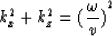$$k_{x}^2+k_{z}^2 = { ( {\omega \over v } ) }^2$$ (1)

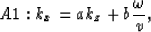
where k_x and k_z are the horizontal and vertical wave-numbers, respectively, and $\omega$ is the temporal frequency. Decomposition of the wavefield into leftgoing (-x) and rightgoing (+x) waves, requires equation (1) to be changed into the following form:

$$k_{x}=\pm \sqrt{ {({\omega \over v})}^2 - k_{z}^2 }$$ (2)

where the positive sign is used for rightgoing, the negative sign for leftgoing waves.

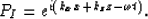
Our starting point is that the total wavefield P_T at the boundary is the sum of the incident wavefield P_I from the interior and the reflected wavefield P_R from the boundary, such that P_T=P_I+P_R. If we let P_T=P_I, then P_R=0, we obtain a perfect nonreflecting boundary. So we use the leftgoing (rightgoing) wave equation as a boundary condition for the left(right) edge. To get difference equations in the space-time domain, we need to rationally approximate equation (2).

Here we give two forms of rational approximation to (2):

$$A1:k_{x}=ak_{z}+b{\omega \over v},$$ (3)

and

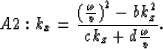$$A2: k_{x}={ { {({\omega \over v})}^2 - bk_{z}^2 } \over { ck_{z} + d{\omega \over v} } }.$$ (4)

In the space-time domain:

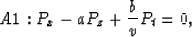$$A1: P_{x}-aP_{z}+{b \over v}P_{t}=0,$$ (5)

and

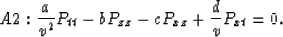$$A2: {a \over v^2}P_{tt}-bP_{zz}-cP_{xz}+{d \over v}P_{xt}=0.$$ (6)

The criterion for the absorbing boundary condition is that it is transparent to the incidence wavefield, that is, the boundary reflection coefficient is very small. Our motivation is to find a boundary condition with a reflection coefficient as small as possible.

Consider a rightgoing plane wave:

$$P_{I}=e^{i(k_{x}x+k_{z}z-\omega t)}.$$ (7)

Suppose the boundary reflection coefficient is R, then the right boundary reflection is:

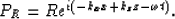$$P_{R}=Re^{i(-k_{x}x+k_{z}z-\omega t)}.$$ (8)

Locally near the boundary, the total wave field P_T=P_I+P_R must satisfy both the boundary condition and the interior wave equation. Applying A2 to (P_I+P_R), we obtain:

$$\vert R\vert=\left\vert{ {bk_{z}^2-a{({\omega \over v})}^2+c... ...})}^2-bk_{z}^2+ck_{x}k_{z}+dk_{x}{\omega \over v}}}\right\vert.$$ (9)

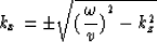
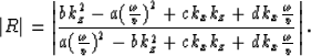
From the interior two-way wave equation dispersion relation, we have:

$${vk_{z} \over \omega}=\sin \theta,$$ (10)

and

$${vk_{x} \over \omega}=\cos \theta.$$ (11)

where $\theta$ is the angle of incidence measured from the normal to the boundary. Then we have:

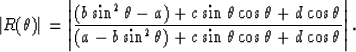$$\vert R(\theta)\vert=\left\vert{ {(b\sin^2\theta-a)+c\sin\th... ...b\sin^2\theta)+c\sin\theta\cos\theta+d\cos\theta} }\right\vert.$$ (12)

In the same way we obtain the reflection coefficient for A1:

$$\vert R(\theta)\vert= \left\vert { {b+a\sin \theta - \cos \theta} \over {b+a\sin \theta + \cos \theta} } \right\vert.$$ (13)

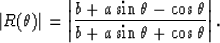
We first give a reflection coefficient R₀=0.1, then by trial and error, we will find a, b, c, and d, so that $\vert R(\theta) \leq R_{0}\vert$ for as many $\theta$as possible. We have

A1: a=-0.55, b=1

A2: a=8, b=8, c=-7.5, d=10.

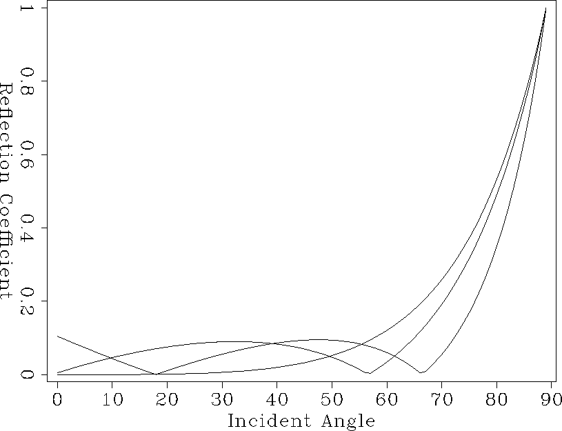
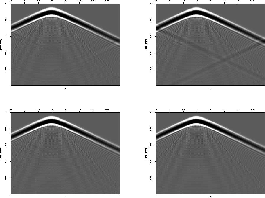
In Figure 1, the reflection coefficients for A1, A2, versus C2 from Clayton et al. (1977) are plotted. The low angle reflection coefficients for A1 and A2 can be decreased, but we have to sacrifice the high angle counterparts. Figure 2 displays the finite difference modeled shot records of different absorbing boundary conditions on the model given by Reynolds (1978, p. 1103).

 

fig1
Figure 1 Graph of reflection coefficients for boundary conditions, A1, A2 versus C2 (Clayton et al. 1977).

 

fig2
Figure 2 Modeled shot records by different absorbing boundary conditions, (a) A1, (b) A2, (c) C2 by Clayton et al. (1977), (d) Reynolds (1978)