Next: CONCLUSION
Up: Ji and Biondi: Explicit
Previous: Lateral velocity variation
For increasing the accuracy at higher dips, we can use more terms
in the Taylor-series expansion. Resulting in a matrix with
thicker bands than the tridiagonal matrix.
Using the second-order term in the expansion, we see that
the approximated square-root operator takes the form
| 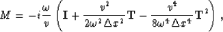 |
(21) |
where I is the identity matrix, and T represents
the tridiagonal matrix that approximates the second partial derivative.
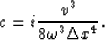
Let
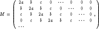
with
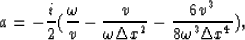
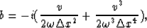
and
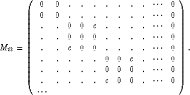
We split the matrix into five pieces, M=Me+Mo+Mt1+Mt2+Mt3,
where
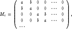
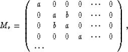
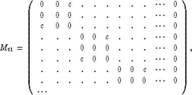
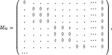
and
In the same manner as the tridiagonal matrix, we can approximate the
time-stepping operator as
|  |
(22) |
Mt1, Mt2, and Mt3 are block diagonal, and
the small block matrix F along the diagonal is defined as
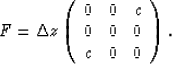
Using the series definition of the exponential function, we see that
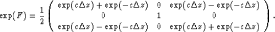
Exponentiating Mt1, Mt2, and Mt3 amounts to
exponentiating F. The terms  ,
, and
and  are also block diagonal.
Since the eigenvalues of
are also block diagonal.
Since the eigenvalues of  are 1 and
  with imaginary c, it follows that
 .As before, to prove the unconditional stability of the algorithm,
we need only show that
.As before, to prove the unconditional stability of the algorithm,
we need only show that
 . This follows immediately since


each of which is equal to 1 according to the preceding argument.
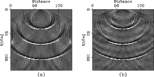
In Figure ![[*]](http://sepwww.stanford.edu/latex2html/cross_ref_motif.gif) , we compared the impulse responses of first-order
approximation with the second-order approximation in the Taylor-series
expansion of the square-root operator.
We also superposed semicircles which is the theoretical solution of
the extrapolation operator on Fig and the higher order
approximation shows better fitting to semicircles than the first-first
order approximation.
, we compared the impulse responses of first-order
approximation with the second-order approximation in the Taylor-series
expansion of the square-root operator.
We also superposed semicircles which is the theoretical solution of
the extrapolation operator on Fig and the higher order
approximation shows better fitting to semicircles than the first-first
order approximation.
With the same manner as showed in this section, we can get more
accurate operator by taking more terms in a Taylor series expansion
of the square-root operator. However, it will produce a matrix
with increasing width of the band and thus will cause to an
increasing in computation cost.
fig3
Figure 3 Impulse response of (a) explicit depth migration with the first-order
approximation for the square-root operator and of (b) explicit depth migration
with the second-order approximation for the square-root operator.


Next: CONCLUSION
Up: Ji and Biondi: Explicit
Previous: Lateral velocity variation
Stanford Exploration Project
12/18/1997