


In the previous example, we inverted for the elastic impedance parameter
set (Ip, Is, ![]() ). However, we could have elected to invert for
any of several other parameter sets: (Vp, Vs,
). However, we could have elected to invert for
any of several other parameter sets: (Vp, Vs, ![]() ) for example.
We have been investigating six parameter sets so far: Impedance
(Ip, Is,
) for example.
We have been investigating six parameter sets so far: Impedance
(Ip, Is, ![]() ), Velocity (Vp, Vs,
), Velocity (Vp, Vs, ![]() ), Elastic Modulus
(
), Elastic Modulus
(![]() ,
, ![]() ,
, ![]() ), Lamé Parameter (
), Lamé Parameter (![]() ,
, ![]() ,
, ![]() ),
Vp/Vs Ratio (Ip, Vp/Vs,
),
Vp/Vs Ratio (Ip, Vp/Vs, ![]() ), and the so-called ``AVO''
Parameters (A, B, C).
In practice, when we are faced with noisy
data given over a limited aperture of specular reflection angles, the
issue of parameter choice can become critical, as we will show.
), and the so-called ``AVO''
Parameters (A, B, C).
In practice, when we are faced with noisy
data given over a limited aperture of specular reflection angles, the
issue of parameter choice can become critical, as we will show.
Figures ![[*]](http://sepwww.stanford.edu/latex2html/cross_ref_motif.gif) and are plots of ``radiation'' curves
for the Impedance
and Velocity parameterizations respectively. A single curve on one plot
(Ip in Figure for example)
is obtained by making a unit perturbation
in that parameter
and are plots of ``radiation'' curves
for the Impedance
and Velocity parameterizations respectively. A single curve on one plot
(Ip in Figure for example)
is obtained by making a unit perturbation
in that parameter ![]() , and setting the other two
parameters in that set to zero
, and setting the other two
parameters in that set to zero ![]() .This yields that parameter's coefficient as a function of specular angle
.This yields that parameter's coefficient as a function of specular angle
![]() from the Bortfeld approximation in the Theory section.
By plotting all three curves for a parameter set we get
Figures or ,
for example.
These curves contain a lot of intuition about how robust
a given parameterization will be.
from the Bortfeld approximation in the Theory section.
By plotting all three curves for a parameter set we get
Figures or ,
for example.
These curves contain a lot of intuition about how robust
a given parameterization will be.
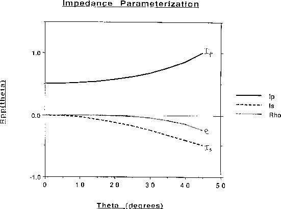
Consider the Impedance radiation curves of Figure . The first thing to
notice is that, in terms of amplitude sensitivity to the data
![]() , Ip is the most sensitive, followed by Is and
lastly
, Ip is the most sensitive, followed by Is and
lastly ![]() . Next, at near offsets Rpp is due only to Ip, which
tends to make it a robust parameter (no ambiguity or non-uniqueness).
As offsets increase to about
. Next, at near offsets Rpp is due only to Ip, which
tends to make it a robust parameter (no ambiguity or non-uniqueness).
As offsets increase to about ![]() , any remaining AVO response in
Rpp not explained by Ip has to be due to Is, since
, any remaining AVO response in
Rpp not explained by Ip has to be due to Is, since ![]() has
zero sensitivity. Hence, the intuition from the radiation curves tells
us that there is a clear order in the robustness of the three parameters,
ranging from Ip the most robust, to
has
zero sensitivity. Hence, the intuition from the radiation curves tells
us that there is a clear order in the robustness of the three parameters,
ranging from Ip the most robust, to ![]() the least robust, that for
the least robust, that for
![]() -
-![]() specular coverage Ip and Is are well resolved, and that
Rpp contains no information about density variations for
specular coverage Ip and Is are well resolved, and that
Rpp contains no information about density variations for ![]() .
.
 |

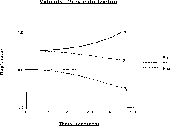 |
In contrast, and to make a point, consider the Velocity radiation curves
of Figure .
At near offsets it is completely ambiguous whether Rpp
is due to changes in Vp or ![]() or both. Worse still, as offsets
increase, the Vs and
or both. Worse still, as offsets
increase, the Vs and ![]() curves are almost parallel. This means
that if a change in Rpp is not explained by Vp with offset, any
inversion scheme will have a difficult time trying to decide if that
change is due to Vs,
curves are almost parallel. This means
that if a change in Rpp is not explained by Vp with offset, any
inversion scheme will have a difficult time trying to decide if that
change is due to Vs, ![]() or both, since they both have the same
change with offset. In noisy, aperture-limited data, the Vp and
or both, since they both have the same
change with offset. In noisy, aperture-limited data, the Vp and
![]() parameters will be closely coupled at near offsets,
and the Vs and
parameters will be closely coupled at near offsets,
and the Vs and ![]() curves will be closely coupled at far offsets
curves will be closely coupled at far offsets
![]() , giving rise to what is called parameter leakage.
, giving rise to what is called parameter leakage.
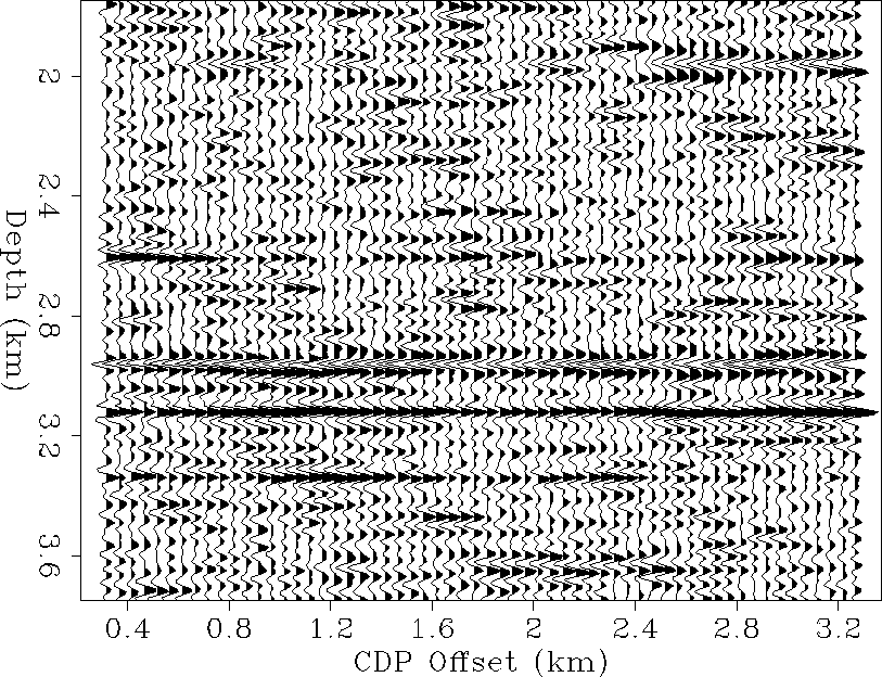
To reinforce this point numerically, we have inverted a noisy version
of our previous synthetic example. Figure is the noisy version of
Figure , obtained by adding random noise, normally distributed with
zero mean and standard deviation equal to one half the near offset
peak gas amplitude at 2960 m (s/n = 2/1 defined), filtered to match the
wavelet frequency band, and with Markovian type lateral coherency.
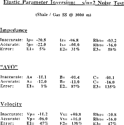
Table gives the inverted elastic parameter estimates for the
Impedance, Velocity, and AVO parameterizations at the shale/gas contact.
The error estimates in
Table are normalized with respect to the
standard deviation of the noise
in the Rpp gather. It is readily evident that our intuitive conclusions
from the radiation curves are justified by the impedance and velocity
inversion results. For comparison, we have also shown the inversion
results with the standard AVO parameterization, which demonstrates a similar
order of accuracy in the A and Ip terms, but an inferior accuracy in the
B term as compared to Is.
This conclusion is intuitively supported by the AVO radiation curves,
which are not shown here.
 |
 |
We are actively developing methods to quantify the optimality of certain
parameter sets in terms of inversion stability, parameter sensitivity, and
parameter accuracy. This work is in preparation for journal publication.
At this point, we recommend the Impedance parameterization for robust
elastic parameter inversion, given reflection data acquired with a specular
angle range of about 0![]() -35
-35![]() .
.