

Next: CONCLUSIONS
Up: A STRUCTURAL SEISMIC MAP
Previous: Tomograms and seismograms
The partial failure of the synthetic seismogram section to reproduce
structural image of the seismic section is caused partly by the presence
of unconformities, which limit the spatial extension of major reflectors,
and also by the lateral changes in the amplitude and shape of
the waveform in a given chronostratigraphic unit.
Both the amplitude and temporal separation of the reflectivities
associated with this unit can change laterally, but the spatial (depth)
pattern is highly uniform, representing the periodic changes
in the depositional environment.
The impression of extensive lateral continuity in a seismic section
comes from the specific patterns in the
impedance transitions, not from the values of the transitions themselves.
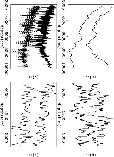
Figure ![[*]](http://sepwww.stanford.edu/latex2html/cross_ref_motif.gif) a shows two of the selected sonic logs. When
looking for similarities between the logs, we can begin by focusing
on their low-wavenumber behavior, as illustrated in
Figure
a shows two of the selected sonic logs. When
looking for similarities between the logs, we can begin by focusing
on their low-wavenumber behavior, as illustrated in
Figure ![[*]](http://sepwww.stanford.edu/latex2html/cross_ref_motif.gif) b. We than have two options: to match
amplitudes or to match shapes, each of which leads to a different result.
If we now analyze the behavior of the higher frequency components
of the logs (Figure
b. We than have two options: to match
amplitudes or to match shapes, each of which leads to a different result.
If we now analyze the behavior of the higher frequency components
of the logs (Figure ![[*]](http://sepwww.stanford.edu/latex2html/cross_ref_motif.gif) c), it becomes
harder to find a match between the logs. A new look at
c), it becomes
harder to find a match between the logs. A new look at ![[*]](http://sepwww.stanford.edu/latex2html/cross_ref_motif.gif) a
reveals that there are different patterns in the high frequency
behavior, with strong oscillations in some parts, ``silent" zones (almost
without oscillations), and some parts where the oscillations are
predominantly to one side of the median.
a
reveals that there are different patterns in the high frequency
behavior, with strong oscillations in some parts, ``silent" zones (almost
without oscillations), and some parts where the oscillations are
predominantly to one side of the median.
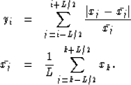
To measure the degree of local variability of the logs, I used a filter
that has the following form:
|  |
(1) |
| |
The output is a measure of the relative variation of the input
inside a window of length L.
To keep a more linear relation between the amplitude of oscillation and
the filter's output, equation (1) uses the absolute value
instead of the usual definition of variation (difference between squares).
Figure ![[*]](http://sepwww.stanford.edu/latex2html/cross_ref_motif.gif) d corresponds to the output of the variability
estimation filter applied to the same part of the logs as that represented
in
d corresponds to the output of the variability
estimation filter applied to the same part of the logs as that represented
in ![[*]](http://sepwww.stanford.edu/latex2html/cross_ref_motif.gif) c. Clearly, the logs in
c. Clearly, the logs in ![[*]](http://sepwww.stanford.edu/latex2html/cross_ref_motif.gif) d can be correlated better
than the logs in
d can be correlated better
than the logs in ![[*]](http://sepwww.stanford.edu/latex2html/cross_ref_motif.gif) c.
four
c.
four
Figure 5 (a) Sonic logs of wells 3476 and 3479 of Figure ![[*]](http://sepwww.stanford.edu/latex2html/cross_ref_motif.gif) .
(b) The same logs after smoothing by convolution with a
triangle (400 points of length). (c) An interval of a
after weak smoothing (40 points triangle). (d) Same interval
of a convolved with a 40 points wide variability filter.
.
(b) The same logs after smoothing by convolution with a
triangle (400 points of length). (c) An interval of a
after weak smoothing (40 points triangle). (d) Same interval
of a convolved with a 40 points wide variability filter.

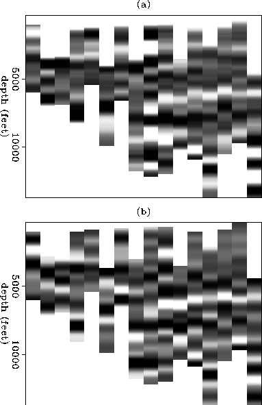
The same filter (using a larger window to avoid spatial aliasing)
was applied to the sixteen wells, the results of which appear in
Figure ![[*]](http://sepwww.stanford.edu/latex2html/cross_ref_motif.gif) b. Figure
b. Figure ![[*]](http://sepwww.stanford.edu/latex2html/cross_ref_motif.gif) a
corresponds to the smoothing of the original logs with a triangle
filter of length equivalent to the the length of the filter applied in
a
corresponds to the smoothing of the original logs with a triangle
filter of length equivalent to the the length of the filter applied in
![[*]](http://sepwww.stanford.edu/latex2html/cross_ref_motif.gif) b.
In both cases, the background trend (very low-frequency components)
was subtracted from the output to emphasize
phase rather than amplitude. The local variability attribute shows
a better lateral correlation over the whole interval than both the
synthetic seismograms and the smoothed logs.
b.
In both cases, the background trend (very low-frequency components)
was subtracted from the output to emphasize
phase rather than amplitude. The local variability attribute shows
a better lateral correlation over the whole interval than both the
synthetic seismograms and the smoothed logs.
allsv1
Figure 6 (a) The logs shown in Figure ![[*]](http://sepwww.stanford.edu/latex2html/cross_ref_motif.gif) a
with subtraction of their strongly smoothed version.
(b) Local variability estimation applied to the original logs.
a
with subtraction of their strongly smoothed version.
(b) Local variability estimation applied to the original logs.


Next: CONCLUSIONS
Up: A STRUCTURAL SEISMIC MAP
Previous: Tomograms and seismograms
Stanford Exploration Project
12/18/1997
![[*]](http://sepwww.stanford.edu/latex2html/cross_ref_motif.gif) a shows two of the selected sonic logs. When
looking for similarities between the logs, we can begin by focusing
on their low-wavenumber behavior, as illustrated in
Figure
a shows two of the selected sonic logs. When
looking for similarities between the logs, we can begin by focusing
on their low-wavenumber behavior, as illustrated in
Figure ![[*]](http://sepwww.stanford.edu/latex2html/cross_ref_motif.gif) b. We than have two options: to match
amplitudes or to match shapes, each of which leads to a different result.
If we now analyze the behavior of the higher frequency components
of the logs (Figure
b. We than have two options: to match
amplitudes or to match shapes, each of which leads to a different result.
If we now analyze the behavior of the higher frequency components
of the logs (Figure ![[*]](http://sepwww.stanford.edu/latex2html/cross_ref_motif.gif) c), it becomes
harder to find a match between the logs. A new look at
c), it becomes
harder to find a match between the logs. A new look at ![[*]](http://sepwww.stanford.edu/latex2html/cross_ref_motif.gif) a
reveals that there are different patterns in the high frequency
behavior, with strong oscillations in some parts, ``silent" zones (almost
without oscillations), and some parts where the oscillations are
predominantly to one side of the median.
a
reveals that there are different patterns in the high frequency
behavior, with strong oscillations in some parts, ``silent" zones (almost
without oscillations), and some parts where the oscillations are
predominantly to one side of the median.


