


Next: WALSH FUNCTIONS
Up: INVERSION SCHEMES
Previous: Nonlinear schemes
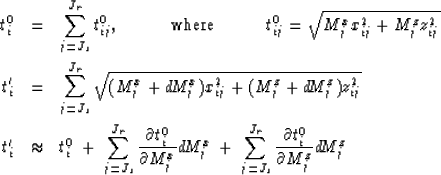
Equation (1) can be linearized for small perturbations around
the homogeneous solution as follows:
|  |
|
| |
| (6) |
Using this approximation in equation (2) and minimizing it
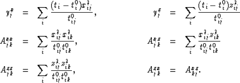
with respect to all  s leads to the following set of linear equations:

where each element  is an
is an  matrix, and
  and
and  are column vectors
with L elements, L being the number of layers (or cells) of the model.
The elements of the matrix and vectors are given by the equations
|  |
(7) |
Michelena (1991) solved the linearized problem using a conjugate gradients
routine. He obtained a stable solution by stopping the process after
a prespecified number of iterations, thus avoiding the problems
arising from the ill-conditioning of matrix  .
Another way to build a more stable algorithm is to introduce an
angle-dependent weighting factor into equation (2) and to
apply a weak constraint to the inversion:
|  |
(8) |
where  is the angle of the ray as measured from the horizontal.


Next: WALSH FUNCTIONS
Up: INVERSION SCHEMES
Previous: Nonlinear schemes
Stanford Exploration Project
12/18/1997


![]()

![]() .
Another way to build a more stable algorithm is to introduce an
angle-dependent weighting factor into equation (2) and to
apply a weak constraint to the inversion:
.
Another way to build a more stable algorithm is to introduce an
angle-dependent weighting factor into equation (2) and to
apply a weak constraint to the inversion:
