Finite-difference method

To use a finite-difference approach, we need to derive formulas for partial derivatives:

$${\partial \hat{x} \over \partial x} \ \ \ \ \hbox{and}\ \ \ \ {\partial \hat{z} \over \partial x},$$

or

$${\partial \hat{x} \over \partial z} \ \ \ \ \hbox{and}\ \ \ \ {\partial \hat{z} \over \partial z}.$$

Let us first simplify notations by denoting

$$\tau(x_c)=\tau(x,z;x_c),\ \ \ \ \hat{\tau}(x_c)=\hat{\tau}(\hat{x},\hat{z};x_c)$$

and

$$\tau_{x_r}(x_c)=\tau_{x_c}(x,z;x_c){\partial x_c \over \part... ...au}_{x_c}(\hat{x},\hat{z};x_c){\partial x_c \over \partial x_r}$$

where x_c=x_s or x_r. Now we define

$$\begin{eqnarray} F(x,z,\hat{x},\hat{z}) & = & \tau(x_s)+\tau(x_r)-\hat{\tau}(x_s... ...x_s)+\tau_{x_r}(x_r)- \hat{\tau}_{x_r}(x_s)-\hat{\tau}_{x_r}(x_r).\end{eqnarray}$$ (6) (7)

Then, equation (5) becomes  

$$\left\{ \begin{array} {l} F(x,z,\hat{x},\hat{z})=0 \\ G(x,z,\hat{x},\hat{z})=0.\end{array}\right.$$ (8)

Taking partial derivative with respect to x on both sides of equation (8) gives:

$$\left\{ \begin{array} {lll} F_x+F_{\hat{x}}\displaystyle{{\p... ...{\partial \hat{z} \over \partial x}} & = & 0.\end{array}\right.$$ (9)

Similarly, taking partial derivative with respect to z yields

$$\left\{ \begin{array} {lll} F_z+F_{\hat{x}}\displaystyle{{\p... ...{\partial \hat{z} \over \partial z}} & = & 0.\end{array}\right.$$ (10)

In matrix notations, these equations become:

$$\pmatrix{ F_{\hat{x}} & F_{\hat{z}} \cr G_{\hat{x}} & ... ...t{z} \over \partial x }} \cr} = -\pmatrix{ F_x \cr G_x \cr }$$ (11)

$$\pmatrix{ F_{\hat{x}} & F_{\hat{z}} \cr G_{\hat{x}} & ... ...t{z} \over \partial z }} \cr} = -\pmatrix{ F_z \cr G_z \cr }.$$ (12)

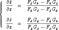
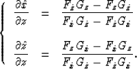
Solving these linear equation sets analytically, we can obtain two sets of partial differential equations for $(\hat{x},\hat{z})$, 

$$\left\{ \begin{array} {lll} \displaystyle{{\partial \hat{x} ... ...\hat{x}}G_{\hat{z}}- F_{\hat{z}}G_{\hat{x}}}}\end{array}\right.$$ (13)

and  

$$\left\{ \begin{array} {lll} \displaystyle{{\partial \hat{x} ... ...hat{x}}G_{\hat{z}}- F_{\hat{z}}G_{\hat{x}}}}.\end{array}\right.$$ (14)

On the right hand side of these equations, we have the partial derivatives of F and G. These partial derivatives are related to the partial derivatives of traveltimes. From equations (6) and (7), we can derive:

$$\begin{array} {lll} F_{\hat{x}} & = & -\hat{\tau}_{\hat{x}}(... ...+\tau_z(x_r)\\ F_z=\tau_{zx_r}(x_s)+\tau_{zx_r}(x_r)\end{array}$$

Because the upwind finite-difference algorithm calculates accurate traveltimes on a regular grid, I use this trave-time table to compute the derivatives of traveltimes, and in turn to compute the expressions on the right hand side of equations (13) and (14). Therefore, equations (13) and (14) become linear partial differential equations and are easy to be solved by many existing numerical algorithms. I use the leapfrog method, in which a partial derivative is taken as a difference between two neighboring points:

$${\partial y \over \partial x} = { y(x+\Delta x)-y(x-\Delta x) \over 2 \Delta x}.$$

To obtain an initial solution, I use searching method to find the operator at some point. The finite-difference algorithm can then calculate the operators elsewhere, and step by step.