TRACE EXTRAPOLATION

The velocity transform ${\bf B}$ comes close to an invertible operator because Radon transforms are theoretically invertible. The velocity transform is a Radon transform with hyperbolic distortion. I think the main invertibility problem stems from numerical approximations in my definition of ${\bf B}$.Unlike ${\bf B}$, operators more typically found in inversion formulations like (2) are both overdetermined and unconstrained. In consequence, I believe we can regard the missing data as the free variables instead of regarding the velocity space $\v$ as the free variables. I'd like to regard the transformation of the complete data space ${\bf x}$to the velocity space $\v$as nearly unitary and noiseless by comparison to that transformation with the truncated data space. Thus in the formulation (2), the first term could be identically zero. Whether this is valid, it is my presumption for the rest of this paper. I presume the problem to be solved is the minimization of the right-hand term in (2). (As we'll see the validity of this assumption is not supported by the field-data trials.)

Happiness is noticing that a problem is much simpler than you had expected. I suddenly realized that the heart of the problem is contained in a much smaller operator than I had thought. Notice that it is computationally easy to decompose integral operators into parts, in this case, into the part of known data and missing data. That is to say, velocity space is The big operator is the one involving the known data ${{\bf B'}_k}$and the little operator is the one involving the few missing traces we will add at the end of the gather ${{\bf B'}_m}$.Both transform to the same plane in velocity space. Thus the regression

$$\bold 0 \quad \approx \quad \v {\quad = \quad}\bar\v + {{\bf B'}_m}{\bf x}_m$$ (7)

involves the ``small'' operator and because it is small, it is reasonable to use many iterations if that should turn out to be helpful.

The idea of minimizing power in image space (velocity space) may be questionable, but makes more intuitive sense when you include a weighting function. Ideally the weighting function would be the inverse of the envelope of the expectation of the variance of the velocity space. In practice we don't know what that is, so I used the envelope of the first estimated velocity space, i.e. that determined from zero padded data. As is common practice I smoothed the envelope and added a constant and experimented with various sized constants.

In practice it happened that few iterations were needed. Convergence appeared to happen on the first iteration.

 

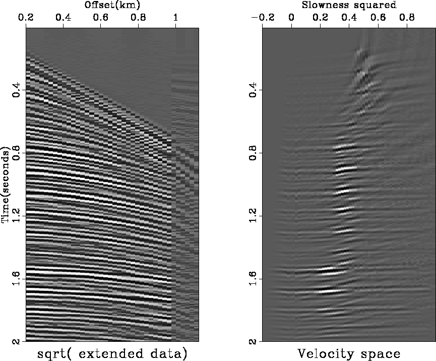
myplot
Figure 1 Attempt to extrapolate a data set.