Flow balancing

 

flow
Figure 1 Flow in a constant velocity medium with a source at the surface in the middle of the model. Flow is shown as 2-D vector fields. The figure shows: (a) the flow variable $\u$, (b) the flux function $F(\u)$, and (c) the vector sum of $\u$ and $F(\u)$.The graphs at the bottom of each plot display the length of the vectors at a constant-depth level in the middle of the model.

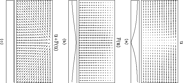
Figure 1 shows the flow variable $\u$ and the flux function $F(\u)$ for a constant-velocity medium. Both are two-dimensional functions, and are drawn as vectors on the 2-D grid, with $\u$, the horizontal time gradient, pointing in the horizontal direction, and $F(\u) = w$, the vertical time gradient, pointing in the vertical direction. The length of the vectors corresponds to the magnitude of the flow. Equation (3) describes the conservation of flow: for each grid cell, the equation balances the change in horizontal flow with the change in vertical flow. Thus, the total flow through each grid cell, the vector sum of $\u$ and $F(\u)$, is constant (Figure 1c). The magnitude of the total flow is s, which denotes the preserved ``substance'' for this problem. (In many fluid-mechanics problems, the flow variable is velocity, and the preserved scalar quantity is energy.)

However, for inhomogeneous media s is not constant, and no classical solution exists. In these media, the flux function F is discontinuous at interfaces where velocity contrasts occur; flow is ``destroyed'' or ``created'' in grid cells along these interfaces. Possible nonclassical solutions to the problem would therefore also be discontinuous: gradient components of the traveltime field would locally obey Snell's law, describing rays that break when passing a velocity contrast.

As discussed before, nonclassical solutions are generally not accessible by finite-difference methods. Instead, viscosity solutions have to be computed, where a numerical ``viscous'' quantity is added to s, which is then preserved by the equation. (In fluid-mechanics problems with energy as the conserved quantity, viscosity allows dissipation of energy.) In computational fluid dynamics, many methods have been developed for computing these viscosity solutions (see Roache, 1976). The next section discusses one particular method.