 |
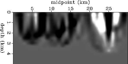
Figure 10 The initial gradient of the stack semblance for the picked events tomographically back-projected into the model space by
 |
Figure 10 shows the initial gradient of the objective function
with respect to the interval slowness model (taken with
![]() ). This plot is the first iteration of
a tomographic back-projection of the
velocity errors.
This gradient gives an idea of what parts of the
model have errors and how changes in those parts of the model
affect the stack semblance of the data.
). This plot is the first iteration of
a tomographic back-projection of the
velocity errors.
This gradient gives an idea of what parts of the
model have errors and how changes in those parts of the model
affect the stack semblance of the data.
 |
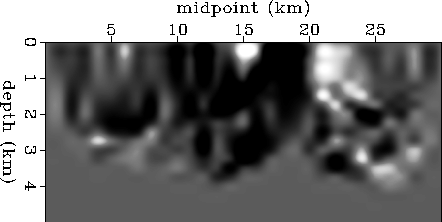
The PARTAN algorithm was run for 30 iterations and stopped
when the gradient of the objective function with respect to
![]() was approximately zero.
Figure 11 shows the cumulative change in the interval slowness model
obtained.
was approximately zero.
Figure 11 shows the cumulative change in the interval slowness model
obtained.