Multiple dips

In most seismic data there are crossing dips present. In order to interpolate this type of data accurately I need an operator that will reject more than one dip. An obvious form for this operator is a cascade of single dip rejection operators. If I wish to reject three dips, p₁,p₂ and p₃, I need an operator of the form,

$${\bf A}_3{\bf A}_2{\bf A}_1 \equiv \left( \frac{\partial}{\p... ...partial}{\partial x} - p_1\frac {\partial}{\partial t} \right).$$

The estimate of the three dominant dips present in the data is found by minimizing the residual,

$$\vert{\bf v}\vert^2 = \vert{\bf A}_3{\bf A}_2{\bf A}_1 \phi \vert^2.$$

Because there are terms involving p₁p₂ etc. this is a nonlinear problem. When linearized for small perturbations in the dip parameters we obtain the following expressions,

$$\Delta v = \sum_{i=1}^3 {\partial v \over \partial p_i} \Delta p$$

In operator form this is

$$\Delta\bold v \ = \ \left[ (\bold A_3 \bold A_2 \delta_t \b... ... \Delta p_1 \\ \Delta p_2 \\ \Delta p_3 \end{array} \right]$$

This expression and the conjugate relationship,

$$\left[ \begin{array} {c} \Delta p_1 \\ \Delta p_2 \\ \Del... ... (\delta_t \bold A_2 \bold A_1 \bold \phi) \end{array} \right]$$

can be used to solve the minimization problem by the method of conjugate gradients.

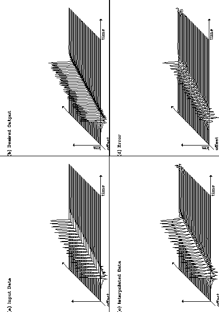
If both the local dip and the missing data values are unknown a non-linear estimation of both the missing data and the local dips can be performed. Figure 9 illustrates the results of applying this process to a simple synthetic with a single dip. In this synthetic every other trace is unknown so the problem is the standard data resampling problem. Panel a) shows the input data and panel b) shows the correct answer, panel c) shows the interpolated output and panel d) shows the difference between the correct answer and the interpolated data. The interpolation has not worked well, the interpolated points are not the same amplitude as the input points, why is this ?

 

altmod1
Figure 9 Wavekill processing of single-dip synthetic. (a) Input data, (b) desired output, (c) interpolated data, (d) difference of (b) and (c).

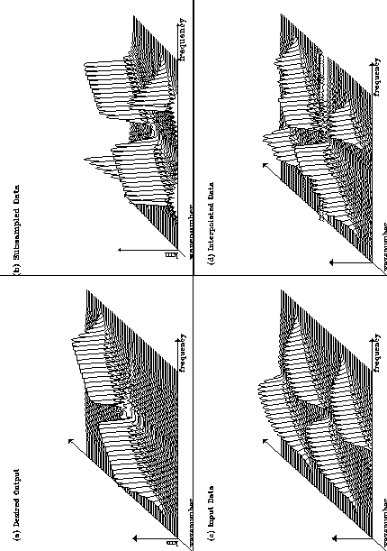
Some insight can be obtained by looking at the data in the $\omega-k_x$ domain. Figure 10 shows four panels transformed into the $\omega-k_x$ domain. Panel a) is the correct answer, panel b) shows the spectrum a dataset that contains every other trace of the correct answer i.e. the known data for the problem. This plot shows that the data is aliased. Panel c) is the spectrum of the known data with zero traces inserted, this is the spectrum of panel b) replicated. This is the initial data that the algorithm uses. The final panel, d), is the spectrum of the interpolated data. There are clearly some artifacts present that are remnants of the aliased, replicated spectrum shown in panel c). When the algorithm chooses the best values of p it is doing so based on aliased data. Because the problem is nonlinear we are not guaranteed to obtain the global solution. Instead the algorithm will find the minimum nearest to the initial solution. In this example the initial solution is that the missing data is zero and the p-values are -1,0,1. The comparison of the desired output spectrum and the spectrum of our initial data proves that this is a poor initial guess.

 

altmodfk1
Figure 10 $\omega-k_x$ plots of wavekill processing of single-dip synthetic. (a) Desired output, (b) spectrum of subsampled data , (c) spectrum of input data, (d) spectrum of interpolated data.

However, this problem is not insurmountable, there is a way to ``bootstrap'' the solution to find a better initial guess. Aliasing is usually only a problem at large $\omega$ and k_x, if I estimate initial values for p using only the unaliased part of the spectrum they should be more reliable than those estimated from the aliased data. I can obtain an unaliased version of the spectrum by smoothing the data in space and time. The smoothing in space and time removes the energy in the spectrum at large $\omega$ and k_x. The fundamental assumption made in using this process is that the dips in the data at low $\omega$ and k_x are the same as the dips present in the correct interpolated output.

I now use a three stage process in interpolating the data:

1.

Smooth the data and estimate initial values for the dips.

2.

Perform a linear estimation of the missing data with fixed dips.

3.

Perform a non-linear, joint estimation of the missing data and dips.

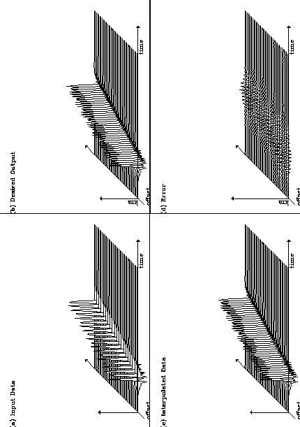
Figure 11 shows the results of applying this three stage process to the single dip synthetic. The interpolated points are much closer to the correct amplitude. Figure 12 shows four spectra. The first is the correct output spectrum, the second is the spectrum of the input data. The third panel shows the spectrum of the smoothed data that is used for the initial estimate of the dips. The last panel shows the spectrum of the interpolated data. The use of better initial values for the dips and the missing data has produced a clearly superior result.

 

altmod2
Figure 11 Bootstrapped wavekill processing of single-dip synthetic. (a) Input data, (b) desired output, (c) interpolated data, (d) difference of (b) and (c).

 

altmodfk2
Figure 12 $\omega-k_x$ plots of wavekill processing of single-dip synthetic. (a) Desired output, (b) Spectrum of input data, (c) Spectrum of smoothed data, (d) Spectrum of interpolated data.

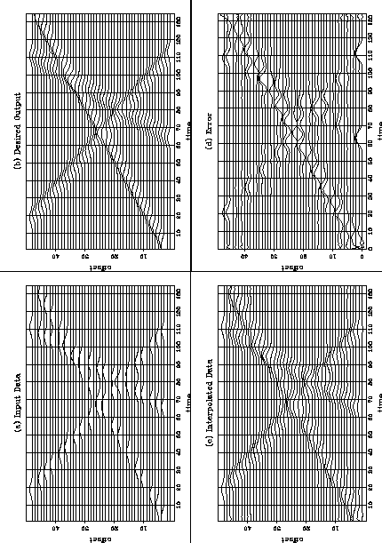
A more complicated synthetic is shown in figures 13 and 14. This is a similar synthetic to the one shown by Spitz(1989). The technique he used is related to the one I have presented. He builds an operator by finding the polynomial representation of a spatial prediction filter in the frequency domain. Once he has found the polynomial he solves for the missing data values. One advantage of the method I have presented is that it is a time domain method. This means that local operators may be constructed by estimating dips within small windows of the data. It is more difficult to construct local operators when working in the frequency domain.

The interpolation of this synthetic is not totally successful as there is still some residual ``jitter'' on the steepest dip. The spectrum of the interpolated data appears to be unaliased but not as extended is $\omega-k_x$ space as the correct answer. It is possible that more iterations are needed to find the correct solution. Another possible solution might be to restart the algorithm and bootstrap it from a smoothed version of the interpolated data.

 

spitz
Figure 13 Bootstrapped wavekill processing of spitz synthetic. (a) Input data, (b) desired output, (c) interpolated data, (d) difference of (b) and (c).

 

spitzfk
Figure 14 $\omega-k_x$ plots of wavekill processing of spitz synthetic. (a) Desired output, (b) Spectrum of input data, (c) Spectrum of smoothed data, (d) Spectrum of interpolated data.

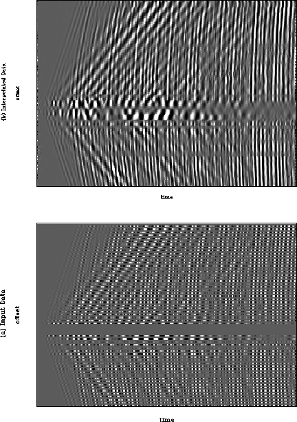
Figure 15 illustrates the application of this four stage process to a real dataset, wz08 (Yilmaz and Cumro, 1983). The dataset has conflicting dips present and a large gap near zero offset. Although the interpolation is unsatisfactory in the gap at zero offset, the rest of the data is well interpolated. The steeply dipping linear events have been correctly interpolated despite the fact that they are aliased at some frequencies.

 

realpext
Figure 15 Bootstrapped wavekill processing of real data (a) Input data, (b) Interpolated output.