next up previous print clean
Next: TWO DIMENSIONAL INTERPOLATION ERROR Up: JOINT ESTIMATION OF OPERATOR Previous: Interpolation Error Filters

Estimation of missing data

To apply the estimation procedure using interpolation error filters I must minimize

\begin{displaymath}
\vert f\,*\,\phi \vert ^2\ =\ \vert f\,*\,u\ +\ f\,*\,k\vert^2 .\end{displaymath}

Since both the filter, f, and the estimated values, u, are model parameters I have a non-linear problem. This problem can be linearized as follows,

\begin{displaymath}
\vert (f_i+\delta f)\,*\,(u_i+\delta u)\ +\ (f_i+\delta f)\,*\,k \vert ^2 \end{displaymath}

\begin{displaymath}
\approx \vert f_i\,*\,( u_i + k ) + \delta f\,*\,( u_i + k ) + f_i\,*\,\delta u \vert^2\end{displaymath}

\begin{displaymath}
= \vert ( u_i + k )\,*\,\delta f\ +\ f_i\,*\,\delta u \ - (\,- f_i\,*\,( u_i + k )\,)\,\vert^2 \end{displaymath}

At each step of the non-linear algorithm I solve the linear problem for the model parameters $\delta u$ and $\delta f$ and then update the estimates of the filter coefficients and missing samples by

\begin{displaymath}
u_{i+1} = u_i + \delta u \ {\rm and }\ f_{i+1} = f_i + \delta f . \end{displaymath}

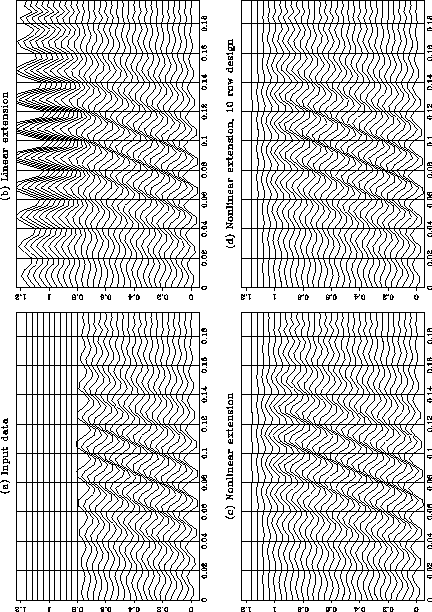
Figure 4 illustrates a case where the linear estimation does not work, there are dips present on the input data. The local smoothness assumption that I made in deriving the linear interpolation process is violated. When I interpolate using the linear operator the dips are not preserved, as seen in the second panel. The nonlinear operator shown in the third panel preserves the spatial spectrum of the input time slices and therefore preserves the dip in the interpolated region. The fourth panel shows the results for the case where the filter is designed on a 10 row window of the data. This should ensure stability in cases where there is noise present in the input.
 
plotnl1
plotnl1
Figure 4
Linear vs. Nonlinear estimation (a) Input data, (b) Linear interpolation, (c) Nonlinear interpolation one row at a time, (d) Nonlinear interpolation, filters designed on a 10 row window.
view

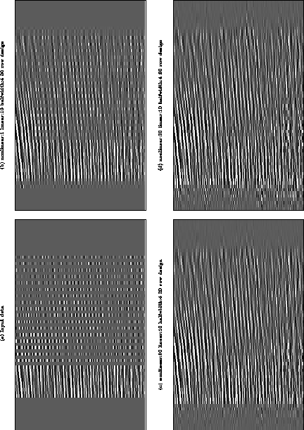
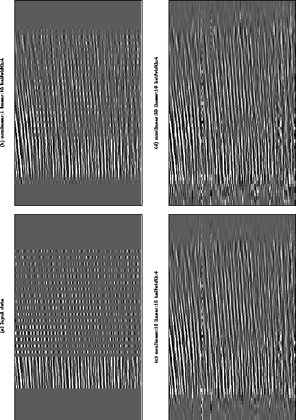
Figure 5 shows the results of applying the nonlinear process to real data. The results generally improve as more nonlinear iterations are performed. Some time slices have extensions that appear to have a different character to the neighboring time slices. This is caused by anomalous amplitudes in the input data. If I stabilize the filter design by estimating it on 20 rows at a time I obtain the more uniform results shown in figure 6
 
plotnl2
plotnl2
Figure 5
Nonlinear estimation with filter of half width 4. (a) Input data, (b) 1 nonlinear step, (c) 10 nonlinear steps, (d) 30 nonlinear steps.
view

 
plotnl3
plotnl3
Figure 6
Nonlinear estimation with filter of half width 4, filters designed on 20 row windows. (a) Input data, (b) 1 iteration of conjugate gradient, (c) 10 iterations, (d) 30 iterations.
view


next up previous print clean
Next: TWO DIMENSIONAL INTERPOLATION ERROR Up: JOINT ESTIMATION OF OPERATOR Previous: Interpolation Error Filters
Stanford Exploration Project
1/13/1998