![]()
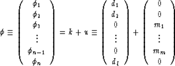
I define two new vectors k and u. The known data, k, is a vector of length n with zeros in place of the unknown values. The unknown data, u, is a vector of length n with zeros is place of the known values. Then,

The objective function I minimize is
![]()
One simple example of a suitable linear operator is a roughening operator. The model that this implies is that the output should be locally smooth.
If I have a smoothing operator, SM, I can define a roughening operator, R = 1 - SM. The residual vector that I want to minimize is ![]() .
.
Many numerical methods can be used to solve this problem. I choose to use a simple conjugate-gradient algorithm ( Claerbout, 1985). The smoothing operator I use is the triangular smoothing operator "Triconv" described by Claerbout(1989). The adjustable parameters in the interpolation algorithm are the length of the smoothing operator and the number of iterations of the conjugate gradient algorithm.
An important property of this type of interpolation method is that it can be used to estimate extensions off the ends of a dataset. If I had simply designed a filter from the input data and then used the filter to predict off the end of the data it might have produced a diverging solution.
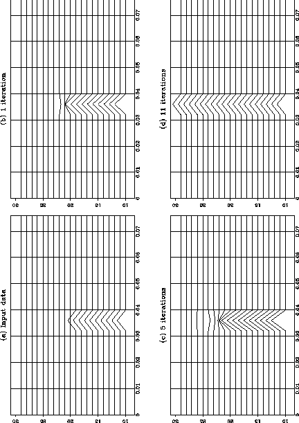
When processing a seismic dataset I treat each time slice independently. This produces one-dimensional vectors of data with unknown samples can be processed using the method described above. Figure 1 shows the processing of a synthetic dataset. The input (a) has equal amplitude spikes across half the gather. Panels (b), (c) and (d) show the results as more iterations of the conjugate gradient algorithm are performed.
 |
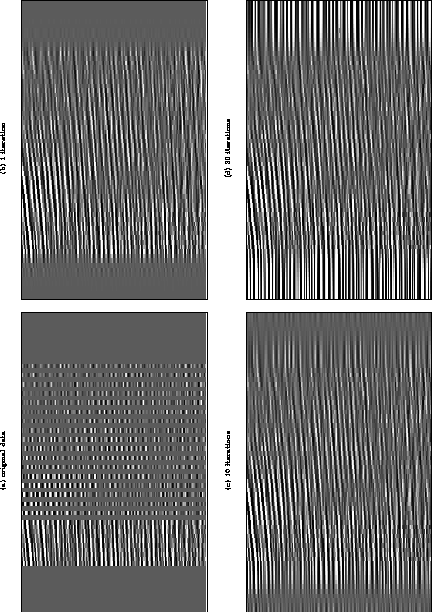
Figures 2 and 3 show the processing of a real dataset. A dataset with half the traces missing at far offsets, wz27 (Yilmaz and Cumro,1983), has been windowed to provide a small test dataset. Normal moveout was applied to the data with water velocity. This has made most events reasonably, but not totally, flat. Figure 2 shows the results of processing with a filter of half width 3 samples. The missing traces at far offsets are well interpolated but as the iterations progress, more energy is put in flat extensions at the ends of the data. This is because the algorithm tries to produce a smooth answer on each time slice separately, and the flat extensions are certainly smooth. Figure 3 shows the results of processing with a filter of half width 7 samples. Because the data has some residual dip it is not smooth over a length of 15 samples. The algorithm only interpolates large amplitudes when it is surrounded by data that is smooth over the length of the filter. Because of the residual dip the results for a longer filter are less successful.
 |
 |
A better approach to the problem might be to avoid any assumptions about the desired output spectrum and instead use an error filter that matches the spectral characteristics of the input data.