


Next: CONCLUSIONS
Up: Gilles Darche: L Deconvolution
Previous: EXAMPLE ON REAL DATA
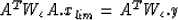
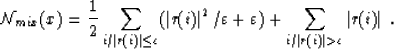
Though the theoretical problem is a Lp norm minimization, the introduction of
the parameter  changes the theoretical resolution. In fact, the limit
xlim of the algorithm will solve the normal equations:
changes the theoretical resolution. In fact, the limit
xlim of the algorithm will solve the normal equations:
|  |
(10) |
where:
r(i) = (y - A.x)(i)
| 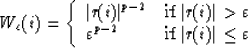 |
(11) |
These equations are the normal equations of the next minimization problem:
| 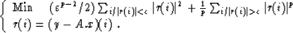 |
(12) |
Effectively, if  , a small perturbation of x will
maintain this inequality, because of the continuity of the matricial product.
This property also holds for the other inequality:
, a small perturbation of x will
maintain this inequality, because of the continuity of the matricial product.
This property also holds for the other inequality:  .It is no longer true if we take large inequalities (
 or
or  ).
So, we can calculate the gradient of the objective function in equation (12)
and keep the same inequalities; if I call this function
).
So, we can calculate the gradient of the objective function in equation (12)
and keep the same inequalities; if I call this function  , then:
| 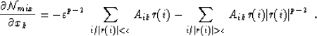 |
(13) |
Finally, replacing r(i) by (y - A.x)(i), we find the normal equations (10).
This result is true if the objective function is minimized for a vector x such that none of the residuals |r(i)| is
equal to .
So, the IRLS algorithm minimizes what would be called a mixed function.
But this objective function is not convex: the summation
of any two vectors x and x' can completely modify the repartition between
residuals larger or smaller than if these vectors are not close
to each other. In fact, this function is strictly convex inside the regions
limited by the 2*ny hyperplanes:

and it is not continuous on these hyperplanes. On
Figure ![[*]](http://sepwww.stanford.edu/latex2html/cross_ref_motif.gif) , I plotted for example the function:
, I plotted for example the function:
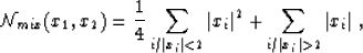
for |xi|<4, obtained with p=1 and =2. This kind of function
has one global minimum, and no other local minimum. However, if we cross the
hyperplanes to reach the region of the global minimum, there might be problems
of computation of the gradient near these hyperplanes, and so problems of
convergence. This problem does not appear with the IRLS algorithm and the
L1 norm, because is small: the central region is smaller,
and the discontinuity (whose jump is proportional to ) becomes
negligible. In fact, the fewer hyperplanes are crossed during the algorithm,
the more efficient the convergence will be. Thus, it is better to have
from the beginning as many residuals as possible smaller than ;that is why the use of a first estimate of the filter enhances the convergence,
and too small an hinders it.
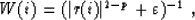
There is in fact another reason which explains the slowness of the convergence
of the IRLS algorithm for a small . A theoretical
n-component L1 solution must produce at least n residuals equal to
zero. But during the algorithm, if any of the residuals gets
smaller than , it creates a weight  for the
next iteration. If is small, this weight will be relatively
large, and will force the same residual, at the next iteration, to be smaller
than . Thus, the algorithm tries to keep this residual small,
independently of whether or not it belongs to the set of theoretical zero
residuals, and we might need many iterations to force the algorithm to
``forget'' this residual.
for the
next iteration. If is small, this weight will be relatively
large, and will force the same residual, at the next iteration, to be smaller
than . Thus, the algorithm tries to keep this residual small,
independently of whether or not it belongs to the set of theoretical zero
residuals, and we might need many iterations to force the algorithm to
``forget'' this residual.
The objective function could be interesting for a mixed
L1-L2 problem, for example, if were taken large enough,
in the minimization problem:
|  |
(14) |
The convergence would be ensured by the proximity of the L2 minimization
problem. Problems of computation of the gradient on the hyperplanes could be
solved by smoothing the objective function near these hyperplanes.
Such a smoothing could be assured by taking:
but this choice would not actually correspond to the same minimization problem.
An intermediate choice would be to assure only the continuity of the objective
function by taking:
The mixed function of the problem (14) could handle two kinds
of noise at the same time: spiky high-amplitude noise with the L1 norm,
and gaussian noise with the L2 norm and the damping factor  .
.
Next: CONCLUSIONS
Up: Gilles Darche: L Deconvolution
Previous: EXAMPLE ON REAL DATA
Stanford Exploration Project
1/13/1998