 |
 |
 |
 | Tomographic full waveform inversion and linear modeling of multiple scattering |  |
![[pdf]](icons/pdf.png) |
Next: Gradient computation with TFWI
Up: Biondi: TFWI and multiple
Previous: Multiple-scattering modeling
We can rewrite
equations 5-6
by performing the following substitution
 |
(12) |
and consequently
 |
(13) |
where  is a convolutional operator
in time that may vary both in space and time;
is a convolutional operator
in time that may vary both in space and time;
 is the identity operator.
For example, when the perturbed wavefield is a
time-shifted version of the background wavefield,
the operator
is a shifted delta function.
With this substitution equation 6
can be rewritten as
is the identity operator.
For example, when the perturbed wavefield is a
time-shifted version of the background wavefield,
the operator
is a shifted delta function.
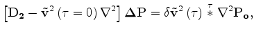
With this substitution equation 6
can be rewritten as
![$\displaystyle \left[ {\bf D_2}- {\bf {v}_o}^2\nabla^2 \right] {\bf {\delta P_o}...
... {v}}}^2\left(\widetilde{\bf T}\stackrel{{t'}}{\ast}{\nabla^2{\bf P_o}}\right),$](img38.png) |
(14) |
where the substitution of
with
 takes into account of the Laplacian.
If we define an velocity model extended in time
 ,
we can rewrite equation 14
as
,
we can rewrite equation 14
as
![$\displaystyle \left[ {\bf D_2}- {\bf {v}_o}^2\nabla^2 \right] {\bf {\delta P_o}...
...\tilde{{v}}}}}^2\left({t},{t'}\right) \stackrel{{t'}}{\ast}{\nabla^2{\bf P_o}}.$](img41.png) |
(15) |
The estimation of an extended velocity as a function of
both  and
and  ,
and for each seismic experiment (e.g. shot), can be unpractical.
We can approximate equation 15
by making the velocity dependent only from the convolutional time lag;
that is,
,
and for each seismic experiment (e.g. shot), can be unpractical.
We can approximate equation 15
by making the velocity dependent only from the convolutional time lag;
that is,
 and the same for each seismic
experiment.
The approximation of equation 15
can be written as
and the same for each seismic
experiment.
The approximation of equation 15
can be written as
 |
(16) |
where the change of notation from
 to
to
 indicates that the scattered wavefield
is now an approximation of
the true multiple-scattered wavefield
.
indicates that the scattered wavefield
is now an approximation of
the true multiple-scattered wavefield
.
Formally solving equation 16
we obtain
![$\displaystyle {\bf {\Delta P}} = \left[ {\bf D_2}- {\bf {\tilde{{v}}}}^2\left({...
...{v}}}}}^2\left({\tau}\right) \stackrel{{\tau}}{\ast}{\nabla^2{\bf P_o}} \right]$](img46.png) |
(17) |
that is a linear relationship between
 and
defined by the linear operator
and
defined by the linear operator
 such as
 .
.
If we define the total wavefield to be
 |
(18) |
and the extended non-linear modeling operator
as
 |
(19) |
the objective function
 |
(20) |
has the same local minima
of the original FWI objective function,
but it also provides
smooth descending paths to the global minimum in the additional dimensions.
The problem is now under constrained because many solutions
fit the data equally well.
Among all these possible solutions we are interested in the solutions
for which the extended velocity model is as focused as possible around
the zero time lag of the model.
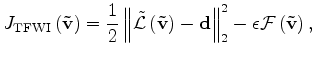
To converge towards a desirable solution we can add
an additional term to the objective function
that penalizes extended velocity model with significant energy
at non-zero time lag;
that is,
 |
(21) |
with
 |
(22) |
where  is an operator that measure the focusing of the model
at zero time lag.
A straightforward example of such operator is
is an operator that measure the focusing of the model
at zero time lag.
A straightforward example of such operator is
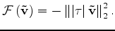 |
(23) |
Subsections
|
|
|
|
| Tomographic full waveform inversion and linear modeling of multiple scattering | |
|
Next: Gradient computation with TFWI
Up: Biondi: TFWI and multiple
Previous: Multiple-scattering modeling
2012-10-29