Early-arrival waveform inversion: Application to cross-well field data

Result analysis

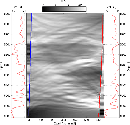
A total of $180$ shots are used. Two passes of inversion are run. First with data bandpassed between $200$ Hz and $400$ Hz, then with data bandpassed between $200$ Hz and $700$ Hz. The final inversion result is shown in Figure 5, with well location indicated by the two slanted lines, and the well velocity value outside the red slanted lines. The inversion result matches well-log data reasonably well, and it better defines the extent of the anomaly, which is also consistent with well-log data. Compared to the tomography result, there are more details in the waveform inversion results. There are some thin layers that are present in the well-log and waveform inversion results, yet are missing in the traveltime tomography result.

invmod
Figure 5. Final model after waveform inversion. Left line is receiver well. Right line is source well. Outside wells are well-log velocity values.

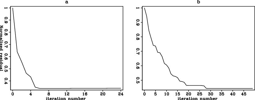
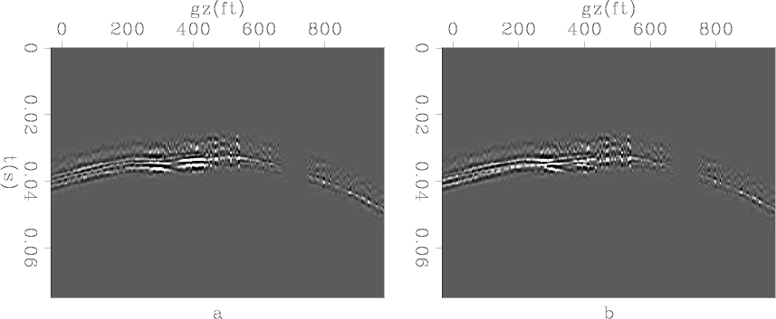
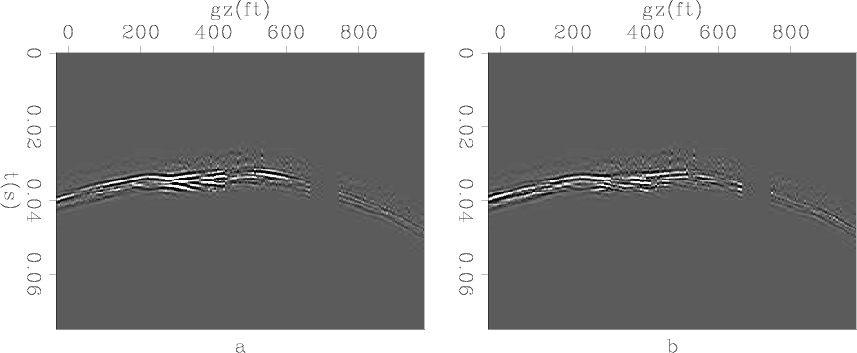
RMS data residual as a function of iteration numbers is shown in Figure 6. Since the initial model is already quite close to the true model, the RMS data residual did not reduce as drastically as expected. A typical shot-gather residual is shown in Figure 7 and 8. It can be seen that data residuals have been reduced mostly in the center part, where rays do not describe the kinematics well.

resd
Figure 6. Data residual of the two inversion steps. a): Normalized residual of 200-400 Hz inversion. b): Normalized residual of 200-700Hz inversion.

rdfulf
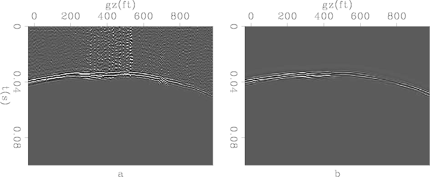
Figure 7. Shot residual of the first inversion steps. a): initial residual. b): final residual.

rdful
Figure 8. Shot residual of the second inversion steps. a): initial residual. b): final residual.

Comparing the forward-modeled first arrival from the initial velocity, the forward-modeled first arrival from the final velocity, and the input first arrival (Fig 4 and 9), the major improvement comes from kinematics matching. This is not surprising, given the inversion objective function we use. The first arrival modeled from initial velocity is continuous, even where the input first arrival is not. Such discontinuity is captured in the first arrival modeled from the final model. Since such discontinuity can be explained better by wave phenomena, ray-based inversion methods can not accurately handle it. Another advantage of waveform inversion is its capability of modeling more than first arrivals. Data modeled from the final velocity predict some later arrivals which do not show up in the data modeled from the initial velocity.

datcomp
Figure 9. Same shot gather as before, comparsion of input first arrival and data modeled from the final inversion result. First arrival modeled from final result matches input kinematics very well. Left: Input first arrival; right: first arrival modeled from the final result.

Early-arrival waveform inversion: Application to cross-well field data