P/S separation of OBS data by inversion in a homogeneous medium

Forward and adjoint isotropic elastic wave propagation

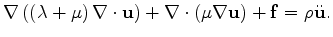
The isotropic elastic wave equation relates displacements to stresses via two elastic constants - the Lam$\acute{e}$ parameters $\lambda$ and $\mu$ :

$$\nabla \left( \left( \lambda + 2\mu \right) \nabla \cdot \mathbf ... ...\left( \mu \nabla \times \mathbf u \right) + \mathbf f = \rho \ddot{\mathbf u},$$ (9)

where $\mathbf u$ are the particle displacements in each dimension, $\mathbf f$ is the force function and $\rho$ is medium density. An alternate formulation is:

$$\nabla \left( \left( \lambda + \mu \right) \nabla \cdot \mathbf u... ... \cdot \left( \mu \nabla \mathbf u \right) + \mathbf f = \rho \ddot{\mathbf u}.$$ (10)

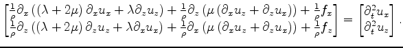
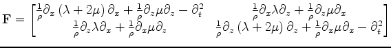
From equation 10, the explicit form for a heterogeneous two dimensional medium can be expressed in a matrix-vector notation as:

$$\begin{bmatrix}\frac{1}{\rho} \partial_x \left( \left( \lambda + ... ...d{bmatrix} = \begin{bmatrix}\partial^2_t u_x \\ \partial^2_t u_z \end{bmatrix}.$$ (11)

The forward elastic propagation operator can then be expressed as:

$$\mathbf F = \begin{bmatrix}\frac{1}{\rho} \partial_x \left( \lamb... ...rtial_z + \frac{1}{\rho} \partial_x \mu \partial_x - \partial^2_t \end{bmatrix}$$ (12)

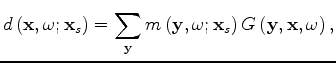
For a homogeneous medium, and using a Green's function to describe the energy propagation between any two locations $\mathbf x = \left( x, y, z \right)$ and $\mathbf y = \left( x, y, z \right)$ , the equation takes the form:

$$\left( \left( \lambda + \mu \right) \nabla \nabla + \mu \nabla^2 ... ...bf x, \mathbf y, \omega \right) = - \delta \left( \mathbf x - \mathbf y \right)$$ (13)

The forward elastic propagation operator injects sources from a model into some location in the medium, and records the resulting wavefield at some other location:

$$d \left( \mathbf x, \omega; \mathbf x_s \right) = \sum_{\mathbf y... ... y, \omega; \mathbf x_s \right) G \left( \mathbf y, \mathbf x, \omega \right) ,$$ (14)

where $m$ is the model of injected sources at location $\mathbf y$ in the medium, and $d$ are the recorded displacement fields $\mathbf u$ at location $\mathbf x$ in the medium. $\omega$ is angular frequency and $\mathbf x_s$ is the shot gather. In vector notation, this is expressed as

$$\mathbf d = \mathbf {Fm},$$ (15)

where $\mathbf F$ is the forward operator. The adjoint operator injects the data from the same recording locations, and records the resulting wavefield at the model injection points:

$$\tilde m \left( \mathbf y, \omega; \mathbf x_s \right) = \sum_{\m... ..., \omega; \mathbf x_s \right) G^* \left( \mathbf x, \mathbf y, \omega \right) ,$$ (16)

which in vector notation is

$$\mathbf {\tilde m} = \mathbf {F^*d},$$ (17)

where $\mathbf F^*$ is the adjoint operator.

P/S separation of OBS data by inversion in a homogeneous medium