Hunting for microseismic reflections using multiplets

Application

The dataset we used in this work was obtained from a monitoring well in the Bossier play (a shale and sand gas reservoir) located in the Dowdy Ranch Field, Texas. The data were collected before (background) and during hydraulic fracture treatments with an array of 12 three-component geophones in a monitoring well. The well was 500ft away from the treatment well (Sharma et al., 2008). The data used in this report are from hydraulic fracture treatment of the Bonner sand formation in this field.

A sonic log has been supplied to us with the data to aid interpretations. As can be seen on Figure 1, there are a couple of strong velocity contrasts that could produce moderately strong reflections.

velnoha Figure 1. Velocity from a sonic log in the monitoring well.

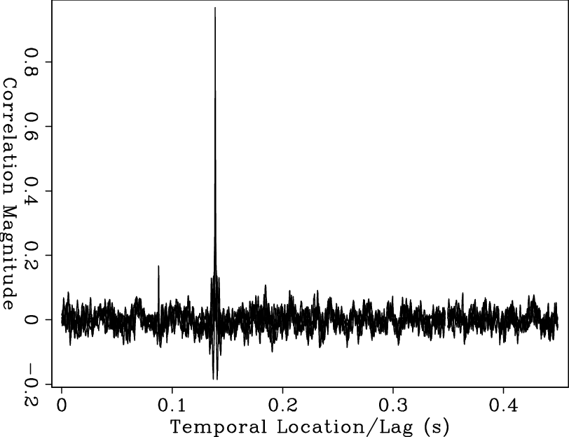
Figure 2 shows a seismogram used for the generation of a master waveform. The waveform between 0.14 and 0.19 s (Figure 3) was extracted from the original seismogram. Normalized cross-correlations of this master waveform with other 0.5 s event windows in the dataset was performed. An example cross-correlation peak of the master with the event window from which it was obtained is shown in Figure 4. The stacked cross-correlation of the peak shown in Figure 4 can be seen in Figure 6(a).

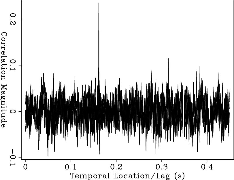
The correlation of the master with another event window is shown in Figure 5. The correlation is stacked (Fig. 6(b)), and the peak location used as detailed below to align this record with that from which the master was extracted.

Bonner0040
Figure 2. Seismogram used in the generation of the master waveform in Figure 3, showing both P and S arrivals.

B0040ma
Figure 3. Master waveform extracted from Figure 2 by windowing in time around 0.14 and 0.19 s.

B40tct40
Figure 4. Cross-correlation of the master with its original event window (Figure 2).The correlation peak is marked

B42tct40
Figure 5. Cross-correlation of the master with another event window with the correlation peak marked

B40tcsti40,B42tcsti40
Figure 6. a) Stack of the correlation in Figure 4. The peak correlation value of 1 reflects the fact that the master window was extracted from the same record. b) Stack of the correlation in Figure 5. Here the peak correlation of 0.24 stands out above the background level of 0.05-0.1.

We used the magnitude of the background correlation of Figures 4 and 5 to set our threshold (minimum) cross-correlation value for multiplet detection. Events that had cross-correlation magnitudes equal to or exceeding this threshold were considered matches/multiplets and used for alignment and stacking. By alignment, we mean that matching waveforms are shifted so that, within the 0.5s event windows they are in, they occur at the same temporal location. This was achieved by applying a bulk positive or negative shift to each event window. The shift for each event window containing a multiplet was the difference in temporal location of the master waveform location and the location of the cross-correlation peak rounded to the nearest sample. After alignment the events were summed together, as shown in Figure 7.

stack3
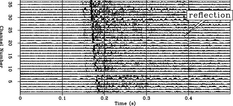
Figure 7. Stacked multiplets for the waveform in Figure 2 with the S reflection marked.

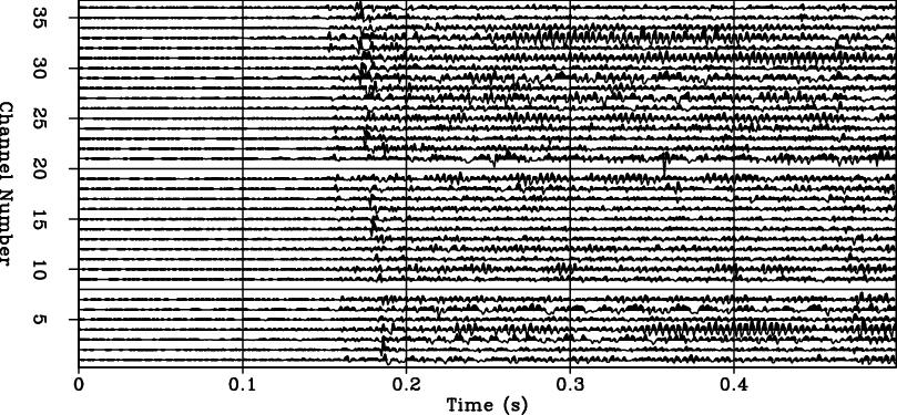
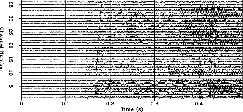
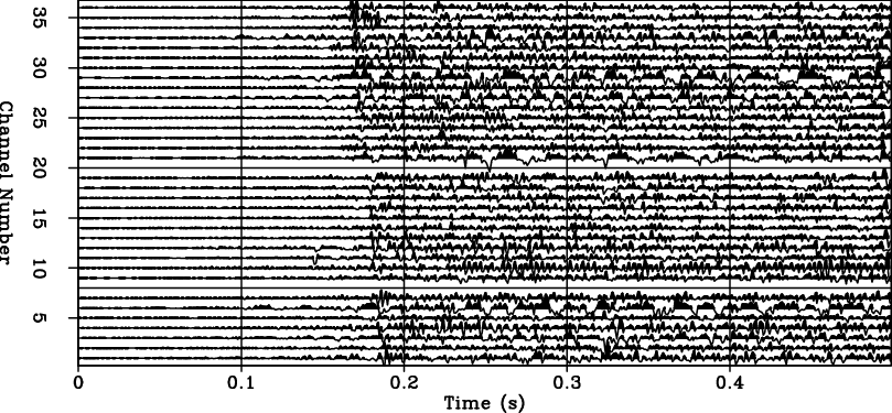
Figure 7 shows stacked traces for the master taken from the seismogram shown in Figure 2. It is clear on the stacked event that the main waveform is followed by another wavelet around 0.39s that was not apparent in the original file from which the master waveform was taken. The event did show up almost consistently at the same temporal offset in most events in the multiplet used to generate this stacked event, as shown in Figures 8-11.

Bonner0455s
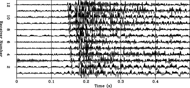
Figure 8. One of the seismograms used in making the stack in Figure 7.

Bonner0152s
Figure 9. One of the seismograms used in making the stack in Figure 7 showing the S reflection.

Bonner0209s
Figure 10. One of the seismograms used in making the stack in Figure 7 showing the S reflection.

Bonner0480s
Figure 11. One of the seismograms used in making the stack in Figure 7 showing the S reflection.

We performed singular value polarization analysis for this stack of events (see the appendix for details) and used this information to emphasize reflection type (S or P). We projected the stacked events using this direction vector to boost P arrivals and possibly see otherwise invisible P reflections. The result of this product is displayed in Figure 12. Comparing this figure with figure 7, we can see that this P-projection has indeed supressed the shear reflection at 0.39s. The S direct arrival was decreased in RMS by a factor of 1.5 and in maximum amplitude by a factor of 3. This projection also increased the P direct arrival RMS by a factor of 1.4.

pboost3
Figure 12. Stack in Figure 7 projected onto the estimated P-direction. When compared to Figure 7, reduction in S amplitude and P amplitude enhancement can be noticed.

As another example, Figures 13-19 exhibit a reflection at about 0.43s for a different master.

Stack0417
Figure 13. The stack of multiplets shown in Figure 14-19 with the S reflection marked.

Bonner0130
Figure 14. One of the seismograms used in making the stack in Figure 13.

Bonner0108
Figure 15. One of the seismograms used in making the stack in Figure 13.

Bonner0097
Figure 16. One of the seismograms used in making the stack in Figure 13.

Bonner0131
Figure 17. One of the seismograms used in making the stack in Figure 13.

Bonner0962
Figure 18. One of the seismograms used in making the stack in Figure 13.

Bonner4211
Figure 19. One of the seismograms used in making the stack in Figure 13.

Hunting for microseismic reflections using multiplets