Tomographic full waveform inversion: Practical and computationally feasible approach

Marmousi Model

A modified Marmousi model is used for the next synthetic example where 500m of water layer is added to the top. Figure 7 shows the true velocity model. A Ricker wavelet with a fundamental frequency of 15 Hz and temporal sampling of 1.5 ms is used as a source function to model the data. There are 461 fixed receivers with a spacing of 20 m and 93 sources with a spacing of 100 m. The initial model is shown in Figure 8 which is obtained by strongly smoothing the true model laterally. The conventional FWI fails when starting from this initial model (Biondi and Almomin, 2012).

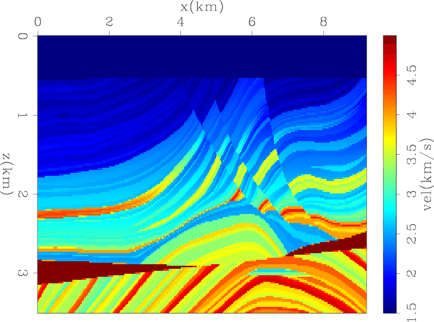
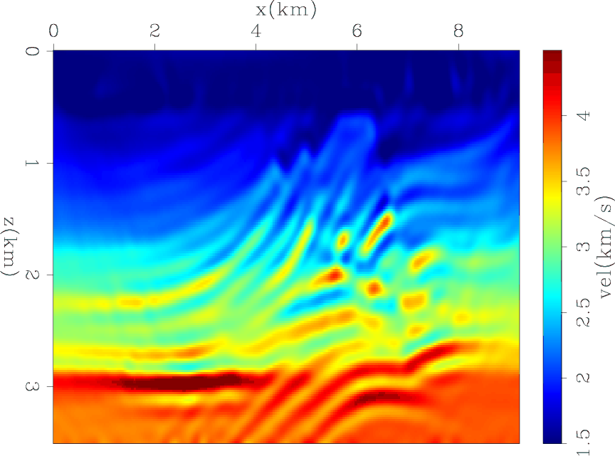
vtrue2
Figure 7. The true velocity of marmousi model.

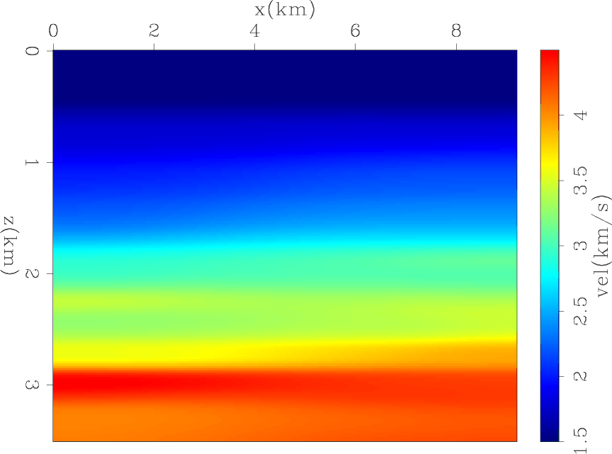
Similar to the Gaussian model, we modeled the observed data with the conventional acoustic wave-equation nonlinear modeling operator. Then, we computed the initial data using the same nonlinear operator on the initial model shown in Figure 8. The two datasets are subtracted from each other to remove the direct arrivals. We then use the subtracted data as the ``observed data" in equation 10.

init
Figure 8. The initial velocity of marmousi model.

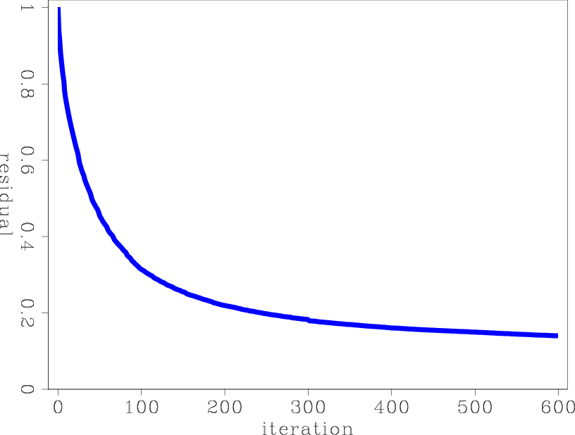
resn Figure 9. The data residual norm as a function of iterations of marmousi model inversion.

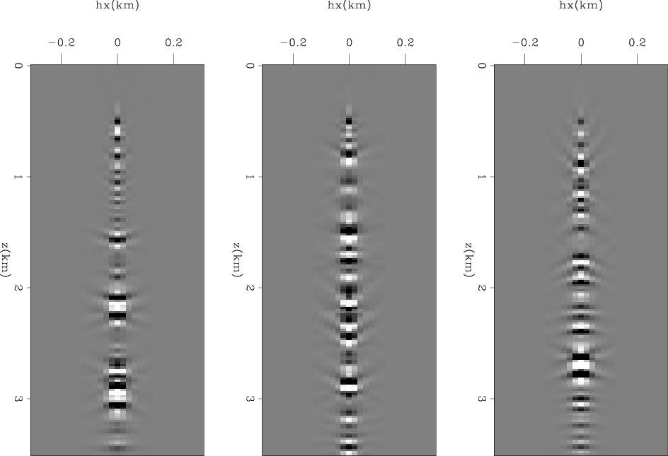
invdv
Figure 10. Three offset-domain common-image gathers of the inverted reflectivity model at x=2.5, 5, 7.5 km of marmousi model.

We show the results of running 600 iterations of minimizing equation 10 where the gradients are mixed as described in equations 16 and 17. Figure 9 shows the normalized residual of the data fitting part, described by the first term of equation 10, as a function of iterations. The residuals decrease monotonically without getting stuck in a local minima. Figure 10 shows three constant-location sections of the final reflectivity model that are a function of depth and subsurface offset. The three images are focused around the middle, i.e. the zero subsurface offset, which indicates convergence towards the correct background model.

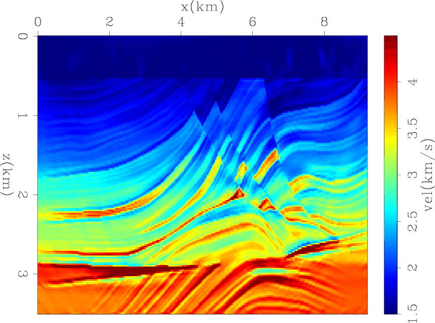
invv
Figure 11. The inverted background of marmousi model.

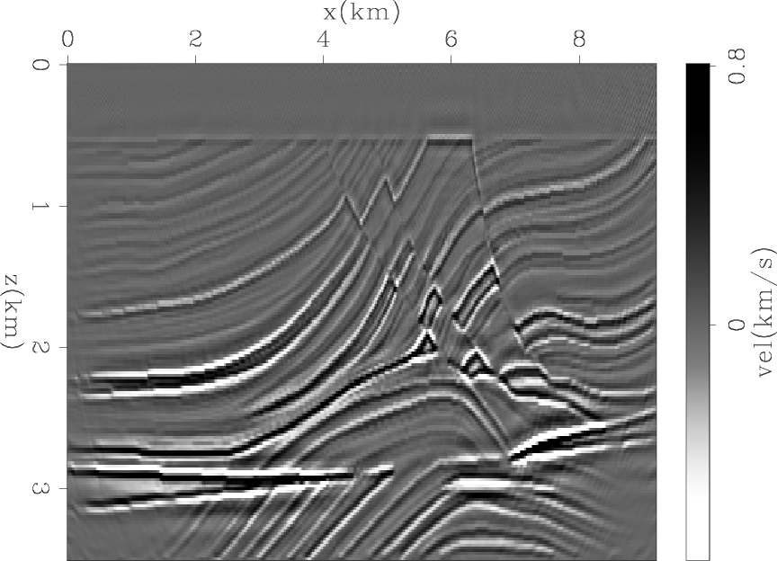
invr1
Figure 12. The inverted reflectivity at h=0 of marmousi model.

inv
Figure 13. The total inversion results of marmousi model.

Figure 11 shows the final background model. It shows great resolution in both the vertical and horizontal directions that captures the main features of the true model. Figure 12 shows zero subsurface offset of the final reflectivity model. Finally, Figure 13 shows the total inverted model which is the sum of the background and reflectivity. It shows remarkable convergence towards the true model.

Tomographic full waveform inversion: Practical and computationally feasible approach