|
|
|
|
A new algorithm for bidirectional deconvolution |
If we assume the the nonlinear part
![]() is relatively
small, we can neglect this term:
is relatively
small, we can neglect this term:
We use matrix algebraic notation to rewrite the fitting
goal. We also want to guarantee filter ![]() to be causal and filter
to be causal and filter ![]() to
be anti-causal during the iterations. For
this we need mask matrices (diagonal matrices with ones on the
diagonal where variables are free and zeros where they are
constrained). The free-mask matrix for
to
be anti-causal during the iterations. For
this we need mask matrices (diagonal matrices with ones on the
diagonal where variables are free and zeros where they are
constrained). The free-mask matrix for ![]() is denoted K, whose first diagonal element is zero, and
that for
is denoted K, whose first diagonal element is zero, and
that for
![]() is denoted Y, whose last diagonal element is zero:
is denoted Y, whose last diagonal element is zero:
From equation (4), we have our new model
![$ {\mathbf{m}} = \left[ {\begin{array}{*{20}c}
{\Delta {\mathbf{b}}^r } & {\Delta {\mathbf{a}}} \\
\par
\end{array} } \right]^T $](img15.png) and new operator
and new operator
![$ {\mathbf{F}} = \left[ {\begin{array}{*{20}c}
{{\mathbf{d}}*{\mathbf{a}}} & {{\mathbf{d}}*{\mathbf{b}}^r } \\
\par
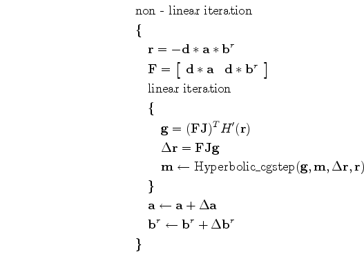
\end{array} } \right]$](img16.png) . Now we can acquire these two filters only by applying the conventional inversion method
and hybrid norm solver. The pseudocode for minimizing this new
objective function by the hyperbolic
conjugate-direction method developed by Claerbout (2010) is:
. Now we can acquire these two filters only by applying the conventional inversion method
and hybrid norm solver. The pseudocode for minimizing this new
objective function by the hyperbolic
conjugate-direction method developed by Claerbout (2010) is:
where
 is defined as the first derivative of the hybrid norm
 is the gradient.
From the template we notice that both linear and non-linear iterations
are needed. Perturbations
![]() and
and
![]() are
inverted by the hyperbolic
conjugate-direction method in each linear iteration. Filters
are
inverted by the hyperbolic
conjugate-direction method in each linear iteration. Filters
![]() and
and
![]() are updated in the non-linear iteration, which generates a new
operator
are updated in the non-linear iteration, which generates a new
operator
![]() to update the model. However, this method requires only
to update the model. However, this method requires only ![]() linear iterations to reach convergence, instead of the
linear iterations to reach convergence, instead of the ![]() linear
iterations required by the previous method, greatly speeding convergence. In addition, there is no need to reverse the filters in
the non-linear iteration, which makes our implementation more convenient.
linear
iterations required by the previous method, greatly speeding convergence. In addition, there is no need to reverse the filters in
the non-linear iteration, which makes our implementation more convenient.
Although the fitting goal is linearized, we still need the initial model to be close enough to get a good result. Here we expect an
impulse function for both filters ![]() and
and ![]() . The following sections
will show the application of this new method and demonstrate its
effectiveness and limitations, when compared with the previous method discussed by Zhang and Claerbout (2010).
. The following sections
will show the application of this new method and demonstrate its
effectiveness and limitations, when compared with the previous method discussed by Zhang and Claerbout (2010).
|
|
|
|
A new algorithm for bidirectional deconvolution |