|
|
|
|
Subsalt imaging by target-oriented wavefield least-squares migration: A 3-D field-data example |
We compute the phase-encoded Hessian using equations 6, 10 and 11.
Since the number of shots is big, we compute only one random realization of the phase-encoded Hessian.
The target region contains ![]() points, with
points, with ![]() samples inline,
samples inline, ![]() crossline and
crossline and ![]() in depth.
The number of elements computed per row for the Hessian is
in depth.
The number of elements computed per row for the Hessian is ![]() (
(![]() in
in ![]() ,
, ![]() in
in ![]() and
and ![]() in
in ![]() ).
Therefore, the widths of the local filter for each image point
are
).
Therefore, the widths of the local filter for each image point
are ![]() km,
km, ![]() km and
km and ![]() km in
km in ![]() ,
, ![]() and
and ![]() directions, respectively.
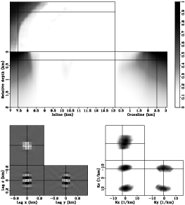
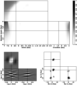
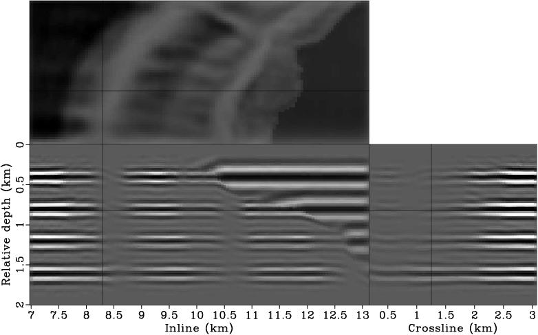
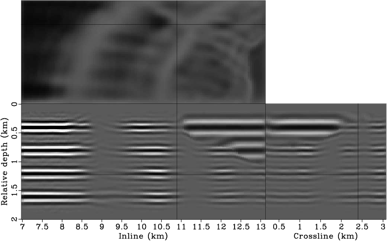
The top panels in Figures 3 and 4 present the diagonal components of
the Hessian matrix at two different slices.
Note that the values of the diagonal of the Hessian are far from uniform, and
the left-side values are much higher than those elsewhere in the
target region. This is because the salt body, which has relatively high velocities,
prevents most of the energy from penetrating itself. The unevenness of the diagonal components also suggests
that the Hessian matrix is highly nonstationary (each row is substantially different than the others).
This is further illustrated by the bottom panels in Figures 3 and 4,
which show the off-diagonal components of the Hessian matrix at two different
image points. For an image point that is well illuminated (bottom panels in Figure 3),
the off-diagonals have relatively wide spectrum coverage and are more focused around the diagonal. On the
other hand, for an image point that is poorly illuminated (bottom panels in Figure 4),
the off-diagonals have relatively narrow spectrum coverage and are more spread in the space domain.
directions, respectively.
The top panels in Figures 3 and 4 present the diagonal components of
the Hessian matrix at two different slices.
Note that the values of the diagonal of the Hessian are far from uniform, and
the left-side values are much higher than those elsewhere in the
target region. This is because the salt body, which has relatively high velocities,
prevents most of the energy from penetrating itself. The unevenness of the diagonal components also suggests
that the Hessian matrix is highly nonstationary (each row is substantially different than the others).
This is further illustrated by the bottom panels in Figures 3 and 4,
which show the off-diagonal components of the Hessian matrix at two different
image points. For an image point that is well illuminated (bottom panels in Figure 3),
the off-diagonals have relatively wide spectrum coverage and are more focused around the diagonal. On the
other hand, for an image point that is poorly illuminated (bottom panels in Figure 4),
the off-diagonals have relatively narrow spectrum coverage and are more spread in the space domain.
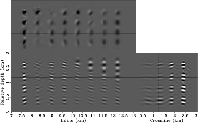
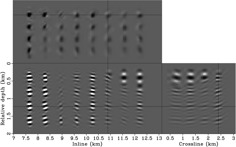
To further appreciate the nonstationarities of the 3-D Hessian matrix, we apply the Hessian to a reflectivity model containing a collection of point scatterers (Figure 5). The result can also be considered as the filter response of the Hessian (where each row can be seen as a filter) to point scatterers. Note how the shape and strength of the filters change across the space. Also note that the filter is more elongated in the crossline direction than in the inline direction. This is a result of the single-azimuth acquisition geometry. Figure 6 shows the Hessian filter response for four horizontal reflectors. Note the imprint of shadow zones on the reflectors. The characteristics of the shadow zones very closely match those in the migrated image (Figure 2), indicating that the computed Hessian matrix, albeit with some approximations, accurately captures the effects of uneven subsurface illumination due to limited acquisition geometry, band-limited wave phenomena and complex overburden. In the subsequent section, I demonstrate how the effects of uneven illumination can be optimally removed by inverting the Hessian matrix through regularized linear inversion.
|
|---|
|
lsm3d-hess-filter1
Figure 3. The Hessian matrix for the target region. The top panel shows the diagonal components of the matrix; the bottom left panel shows the off-diagonals of the matrix taken from the image point at inline |
|
|
|
|---|
|
lsm3d-hess-filter2
Figure 4. The Hessian matrix for the target region. The top panel shows the diagonal components of the matrix; the bottom left panel shows the off-diagonals of the matrix taken from the image point at inline |
|
|
|
|---|
|
lsm3d-imag-spike1,lsm3d-imag-spike2
Figure 5. Hessian filter response for point scatterers. Panels (a) and (b) show different slices of the same 3-D cube. Note the nonstationarity of the filters. [CR] |
|
|
|
|---|
|
lsm3d-imag-flat1,lsm3d-imag-flat2
Figure 6. Hessian filter response for horizontal reflectors. Panels (a) and (b) show different slices of the same 3-D cube. Note the imprint of shadow zones on the reflectors. [CR] |
|
|
|
|
|
|
Subsalt imaging by target-oriented wavefield least-squares migration: A 3-D field-data example |