|
|
|
|
Subsalt imaging by target-oriented wavefield least-squares migration: A 3-D field-data example |
We compute the migrated image using the 3-D conincal-wave migration operator, where we
synthesize ![]() conical waves for each crossline and migrate
conical waves for each crossline and migrate ![]() conical
waves in total. The minimum and maximum inline take-off angles at the surface for the conical waves are
conical
waves in total. The minimum and maximum inline take-off angles at the surface for the conical waves are
![]() and
and ![]() , respectively. The maximum frequency used for migration is
, respectively. The maximum frequency used for migration is ![]() Hz.
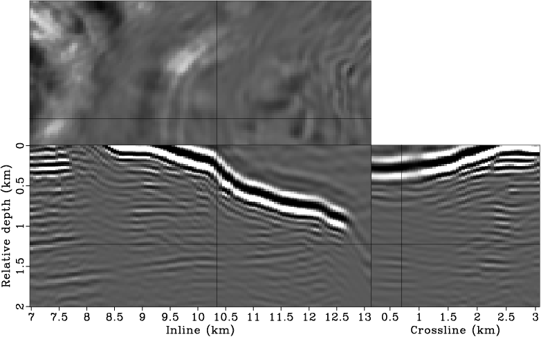
The image obtained for the target area is shown in Figure 2. Note that the amplitudes
of the sediment reflectors are biased; also notice the illumination shadows below the salt due to
the non-unitary characteristic of the Born modeling operator.
Hz.
The image obtained for the target area is shown in Figure 2. Note that the amplitudes
of the sediment reflectors are biased; also notice the illumination shadows below the salt due to
the non-unitary characteristic of the Born modeling operator.
|
|---|
|
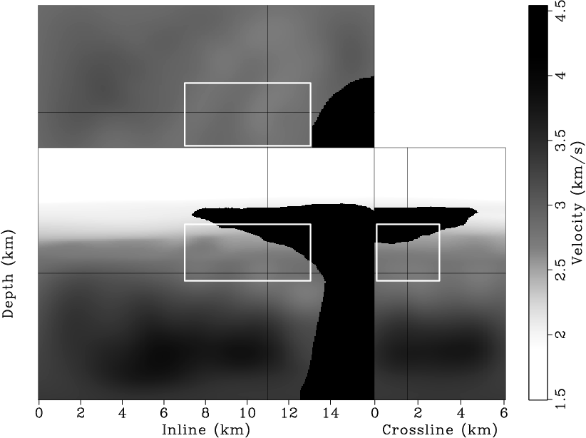
lsm3d-target
Figure 1. Target area selected (outlined by a box) for wavefield least-squares migration. [CR] |
|
|
|
|---|
|
lsm3d-imag
Figure 2. Migrated image for the selected target region. Note the illumination shadows below the salt. [CR] |
|
|
|
|
|
|
Subsalt imaging by target-oriented wavefield least-squares migration: A 3-D field-data example |