|
 |
 |
 | Moveout-based wave-equation migration velocity analysis |  |
![[pdf]](icons/pdf.png) |
Next: Introducing the residual moveout
Up: Theory
Previous: Theory
In this section we present the formula that links the slowness perturbation to the shifts of the ADCIGs.
Starting from the initial slowness model  , we first define the pre-stack common-image gather in the angle domain as
 , where
  is the reflection angle.
If we choose a different slowness
is the reflection angle.
If we choose a different slowness  , the new image
 will be different from
in terms of both kinematics and amplitude. If, as is commonly done, we focus on the kinematic change,
then a way to characterize this kinematic change is to define a shift parameter
will be different from
in terms of both kinematics and amplitude. If, as is commonly done, we focus on the kinematic change,
then a way to characterize this kinematic change is to define a shift parameter  at each image location,
 ,
such that if we apply this shift parameter to the initial image,
the resulting image
,
such that if we apply this shift parameter to the initial image,
the resulting image
 will agree with the new image
in terms of kinematics.
This is indicated by
the maximum point of the auxilary objective function:
will agree with the new image
in terms of kinematics.
This is indicated by
the maximum point of the auxilary objective function:
 for each x,z. for each x,z. |
(1) |
Note that in order to handle multiple events, we use a local window of length 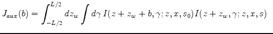 along the depth axis.
For the rest of the paper, the integration bound for variable
along the depth axis.
For the rest of the paper, the integration bound for variable  is always
![$ [-L/2,L/2]$](img21.png) , and each
, and each  is defined within that window around image point (x,z).
 represents a windowed version of the entire image.
This methodology is borrowed from Luo and Schuster (1991) who tried to find the relation of the travel-time perturbation to the slowness change.
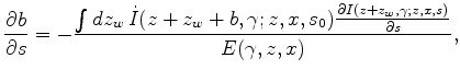
Then
 can be found using the rule of partial derivatvies for implicit functions (please refer to the appendix A):
 |
(2) |
in which
 .
.
 and
and  indicate the first and second derivatives in
  (depth).
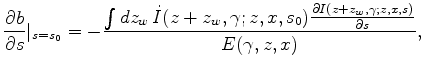
In practice, eq. (2) will be greatly simplified if we evaluate this expression at
(depth).
In practice, eq. (2) will be greatly simplified if we evaluate this expression at  , in other words
  .
In fact, this will always be the case if we update the intial slowness
.
In fact, this will always be the case if we update the intial slowness  after each iteration. The simplified relation becomes
 |
(3) |
and the
 term is indeed the wave-equation image-space tomographic operator.
Each part in eq. (3) has clear physical implications: the
term is indeed the wave-equation image-space tomographic operator.
Each part in eq. (3) has clear physical implications: the 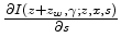 term acts as an energy term to normalize the amplitude of the back-projected image; the back-projected image,
 is built based on the initial image; it also has a first-order
derivative that introduces a proper
is built based on the initial image; it also has a first-order
derivative that introduces a proper  phase shift, ensuring a well behaved slowness update from the tomographic operator.
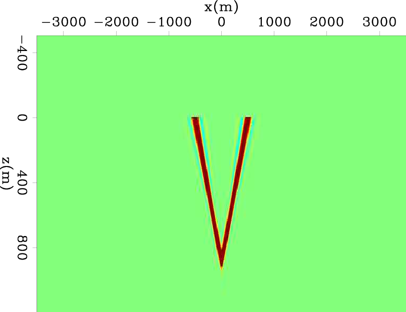
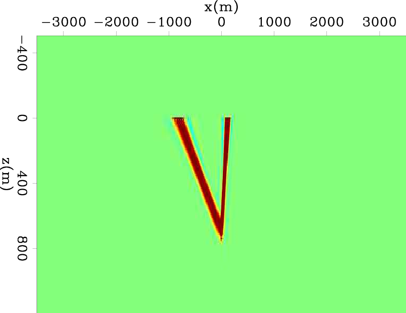
For a simple illustration of eq. (3), the slowness sensitivity kernel is calculated,
by back-projecting a shift perturbation
 that has one single spike at
 .
A uniform background velocity of 2000 m/s is used.
Figure 1(a) shows the sensitivity kernel if the reflector is flat, and figure 1(b)
shows the sensitivity kernel with a dipping reflector (dip angle =
.
A uniform background velocity of 2000 m/s is used.
Figure 1(a) shows the sensitivity kernel if the reflector is flat, and figure 1(b)
shows the sensitivity kernel with a dipping reflector (dip angle =
 ). As is clearly shown in these two plots, this operator
will project the slowness perturbation along the corresponding wave path based on the location and reflection angle of the image shift.
). As is clearly shown in these two plots, this operator
will project the slowness perturbation along the corresponding wave path based on the location and reflection angle of the image shift.
|
|
|
|
| Moveout-based wave-equation migration velocity analysis | |
|
Next: Introducing the residual moveout
Up: Theory
Previous: Theory
2011-05-24